The best way to understand how Port Phillip Bay's tides behave (or are predicted to behave) is to examine graphs that show how the relative heights both inside and outside the Bay change over time. Such a collection of tide curves show the all main features of the behaviour including the very important "Equal Levels" and "Slack Water" moments. However first some review of how the outside tides are created is in order. Impatient readers might want to skip forward to the first image but then may miss some important points.
Most folk will know that tides in the world's seas and oceans have something to do with the gravity of the Sun and Moon affecting water levels here on Earth. Most boating folk will be aware the Moon's role in this is bigger than that of the Sun by a little over two times. A common explanation, even from teachers, is ". . that although the Moon's mass is so much smaller than the Sun's, it is so very much closer that its gravitational tug on the Earth is stronger than the Sun's".
This is incorrect. If it were true then the Earth's major orbit would be around the Moon rather than the Sun. In fact the Sun's gravitational tug here on the Earth is around 180 times stronger than the Moon's tug on the Earth. So why does the Moon play the more dominant role in raising tides here on Earth?
Well it is not the absolute strength of a celestial body's gravitational tug on the Earth that matters in raising tides here, but rather by how much that tug differs over different parts of the Earth. In other words it is the gradient of the celestial body's gravitational field, not its absolute strength, that is the key factor in creating tides. So while the Sun's tug is so much stronger, its gradient across the Earth is fairly small because those distances are tiny compared to the enormous distance to the Sun. On the other hand, although the Moon's tug is 180 times smaller, it orbits us at such a relatively close range that the gradient of its tug across the Earth is around 2.2 times larger than the gradient in the Sun's gravitational field.
Even when the Moon and Sun's tide raising forces combine best at New moon or Full Moon, they are still very weak at about one ten millionth of the Earth's own gravity. A direct upward "pull" by these forces on the several kilometres deep ocean water directly underneath the Moon can't raise its level anymore than 1 mm. However, from many hundred to several thousands of kilometres in all directions around that point, those weak forces do have a small sideways component directed inwards back towards the centre point directly beneath the Moon. It is far easier to shift water sideways towards the sublunar point rather than to try a direct upward lift.
By these actions over many thousands of square kilometres of ocean surface, the shifted water forms a small low angled mound with its centre directly under the Moon. It rises to 0.5m or less above the average ocean level. At around this height, the increased water pressure under the mound is just sufficient to settle into equilibrium with those inwards forces and so the mound grows no bigger. The water movement that did occur also took water away from all the distant ocean areas where the Moon is seen to be at 30 degrees or lower above the horizon. These areas then experience a dip in their water level. The level difference from the bottom of the dip to the top of the distant mound, still no more than one metre, is known as a deep ocean "tidal bulge".
There are also horizontal components of the tide generating forces on the far side of the Earth that also raise a similar size tidal bulge, exactly opposite the near side sublunar point. In a practical sense the Moon's larger tidal bulges and Sun's smaller ones get combined into a single pair of tidal bulges. Now normally this will no longer be exactly under the Moon, and can also vary in size depending on the changing angle between the Moon and Sun as viewed from Earth. The are also many other smaller astronomical details of the orbits of both bodies that cause small variations in the size and timing of each bulge.
Due to the rotation of the Earth about its axis, our continental shorelines get swept through the pair of tidal bulges and the dips between them. In this process there are usually additional geographic amplifications of the high and low levels as well as timing distortions. These all go into producing a local tide behaviour that is fairly unique in height, timing, character, and range for each different coastal location.
Due to the rotation of the Earth, the daytime Sun appears to sweep westward across the sky, taking 24 hours before we see it arrive back on the same meridian of longitude. Its apparent angular speed across the sky is then 360/24 = 15 degrees per hour towards the west. Of course it looks this way because our location is actually spinning eastward at 15 degrees/hour while the Sun's direction from the Earth's centre only changes slightly over 24 hours.
The Moon takes a little longer between meridian passages because during a 24 hour solar day it moves some 12.2 degrees further eastward due to its movement along its own orbital path. The Earth then has to spin a little further eastward for the Moon to appear back over the same meridian again. The extra time needed is 50 minutes, giving a "lunar day" of 24hrs and 50 minutes. This means that on average the high and low tides occur approximately 50 minutes later each day.
Most boating folk are aware that in cycling through the phases of the Moon their local tide undergoes a significant fortnightly change in range. When the apparent angle between the two is near either 0 degrees (New Moon) or 180 degrees (Full Moon), the lunar bulge is enhanced by the in-phase solar bulge. This gives "spring tides" of higher range. Seven days later when they are near 90 or 270 degrees apart (ie. a First Quarter or Third Quarter Moon), the solar bulge aligns with the lunar dip and so these partially cancel one another out to give smaller range "neap tides".
A point worthy of note here is that while for most places on a coast where the deep ocean water beyond the continental shelf is not too far offshore, the spring tides usually reach their peak range within 1 day or so after a Full or New Moon. However on the Central Victorian Coast, the large and relatively shallow Bass Strait means the true deep ocean water is over 200 kilometres away. The inertia and frictional effects of the shallow water on the Bass Strait plateau means the peak range of its tidal response doesn't occur until 4 or 5 days after a Full Moon or a New Moon.
Given there are only 7 days between spring and neap tides, any boating plans for Port Phillip may need to take into account that neap tides (and weakest currents) occur a few days before a New Moon or a Full Moon, and that spring tides (and strongest currents) occur just a few days before a Quartering Moon. This image shows the neap and spring tide delays at Port Phillip Heads:-

A final point about the fortnightly spring-neap cycle is in regard to tide timing over consecutive days. A common notion is that say any particular tide will occur "about an hour later each day". We know that the Moon takes 24hrs + 50 minutes to arrive back in the same position the next day. At both New and Full Moon, the solar and lunar bulges are well aligned with each other so that when the solar contribution is added in, only the height of the bulge is changed and not its timing. So we expect the time of the high/low tide on that day is close to 50 minutes later than on the previous day.
However in each of the days following a New Moon the solar bulge is taken 50 minutes further westward of the lunar bulge, so when combined with the lunar bulge it pulls the resultant bulge peak a little bit more westward of the Moon's position and a bit closer towards the Sun's position. This means we experience that tide a little less than 50 minutes later than on the previous day. In the days before NM/FM we get the reverse effect with each tide appearing more than 50 minutes later than on the previous day.
Both these timing shifts peak at around 3-5 days before and after NM/FM. The result is that for Port Phillip Heads around neap tides, the tides (and slack water times) are around 60 minutes or more later each day, while near spring tides the day-to-day delay is closer to 30 minutes.
In the case of the Sun, because the Earth's axis of daily rotation is tilted by 23.5 degrees to its axis of revolution around the Sun, it appears to us that its position above the Earth also wonders slowly both north and south across the equator in a band from 23.5 degrees north to 23.5 degrees south. This cycle takes 365.25 days to complete. The Latitude of the sub-solar point is called the solar declination angle. There are two Equator crossings each year at the spring and autumn equinoxes, where the solar declination angle is zero.
The Moon also appears to wander back and forth across the equator but it takes just 27 days for its cycle. The amplitude of its north-south wanderings is a bit trickier because its orbital plane is tilted at 5.1 degrees to the orbital plane of the Earth. In a further complication the axis of the Moon's orbital tilt also slowly changes its direction (precesses) relative to the fixed stars. It takes 18.6 years to return back to the same direction, so the complex tidal patterns here on Earth only repeat closely after every 18.6 years.
Putting all that together means the north-south limits of the Moon's monthly declination swing cycle slowly change over a period of 18.6 years. Once every 18.6 years the tilt in the Moon's orbital plane leans in the same direction as the tilt in the Earth's axis. When this occurs the Moon's monthly declination swing range becomes the sum of the two tilts, or 23.5 + 5.1 = 28.6 degrees north or south of the equator. A little over nine years later the tilts are then in opposite directions, reducing the Moon's declination swing range to just 23.5 - 5.1 = 18.4 degrees north or south of the equator.
The point is relevant here because the time of maximum swing range occurred recently in late 2024. The tidal effects of these larger than average N-S lunar declination swings continue for several years around that time. You may have noticed this extreme range recently. In Melbourne the Moon might have appeared very high in the sky one night at around just 10 degrees off the vertical, yet 14 days later its highest altitude might have reached only 24 degrees above the northern horizon.
The effect on tides when the lunar declination is in the northern hemisphere, particularly during our winter when the Sun is also there, is to drag the near side tidal bulge towards the north, with the far side tidal bulge moving towards the south. In this scenario, as the Earth rotates, some locations on the surface may pass through the higher parts of one bulge, then some 12 hours later through the not so high parts of the opposite bulge. This gives successive high tides of unequal height and also gives successive low tides of unequal height.
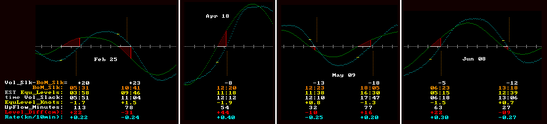
Because this tidal difference happens just once per day, it is referred to as the "diurnal (once a day) inequality". The image below shows 3 cases for the tide curve of a location a few nautical miles outside the Heads. The first graph is from a date where both the Sun and Moon are very close to directly above the equator so successive tides show almost NO diurnal inequality. Graphs #2 & #3 show two extreme cases where both Sun and Moon's declinations are in the same hemisphere and near their maximum possible values, so giving a strong diurnal inequality.
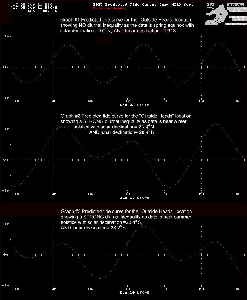
A little over nine years later the two tilts lean in towards each other and so reduce the Moon's monthly declination swing cycle to its minimum range of only 18.4 degrees North or South of the equator. The diurnal inequality is now on a slow downward path to a reduction of 35% by 2034.
The tides outside the Heads can be decomposed into a hundred or more components, each due to some feature of the motion within the Earth-Moon-Sun system and each having a unique cycle period. The major components are grouped around a 12 hour period and are called semi-diurnal (basically twice a day). The diurnal (once a day) components we have just met due to declination swings. There are many other smaller, longer period components. One example is components that reflect the eccentricity of both the Sun and Moon's orbits.
Knowing the amplitudes, periods, and relative phase angles of all the components of each location's tidal signal then allows the tide height to be predicted at any given time. The 6 minute predicted tide heights in these articles are produced by prediction software from the National Tidal Unit, who made available a copy of the Fortran source code and assisted me through the code modifications to suit my modelling work. Their help and assistance is very much appreciated.
In mild and stable weather conditions the real observed tide curves are generally in fair agreement with the predictions. However in very rough weather there can be significant departures from the predicted values. Hopefully these effects might be better understood in the future, but for now the aim is to discover a more accurate picture of how the system "works" in benign weather conditions before probing any further.
The tides in Bass Strait are classified as a "mixed tide" with both semi-diurnal and diurnal components, but is mainly semi-diurnal in character. However the narrow Heads and the large main body of Port Phillip create a "low pass filter" effect which allows the ~24hr diurnal frequency components to pass through the Heads with less attenuation than the ~12hr semi-diurnal ones. Therefore inside the Bay the tide classification changes to "mixed, but mainly diurnal". One consequence of this is that when a strong diurnal inequality is present within the Bay, it leads to a day of highly unequal tidal stream strengths, unequal stream durations, and unequal durations of the slack water periods as the tidal streams reverse.
The satellite view below shows Port Phillip Bay with the three important tidal zones marked in. These assist with the discussion and understanding of the tidal flows through the entrance.
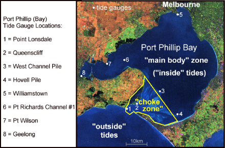
The "outside" tide zone is of course Bass Strait, where the maximum tidal range is up to 2.4 m. The "inside" tide zone comprises the "main body" of the Bay and includes its western arm. This zone has a very large surface area of around 1,700 km2. The maximum tidal range over this vast area is around 0.9 m.
The "choke zone" is sandwiched between the outside and inside zones and is responsible for limiting the rate of water flow between them. Many folk think it is just the narrow gap at the Heads that is the controlling feature that limits inflows and outflows. While there is some truth in this idea when the tidal currents are running fast, at the lower current speeds near the beginning and end of a tidal stream, the dynamic forces needed to accelerate and decelerate the large moving water mass come into play. Since a lot of the water mass is concentrated in the wider parts of the "choke zone", much of the "flow resistance" due to dynamic forces makes the area between Queenscliff and the Hovell Pile/ or the West Channel Pile important approaching slack water. This will be seen later on when tide plots across the "choke zone" are shown.
The plot below shows the red "outside" tide height over time for the first of May 2025. Also shown are the "inside" tide curves at four different colour coded locations within the Bay's main body zone. The white graduations along the horizontal axis are at 1 hour intervals. The marks and numbers further down and just above the date identify 6 hour time intervals.
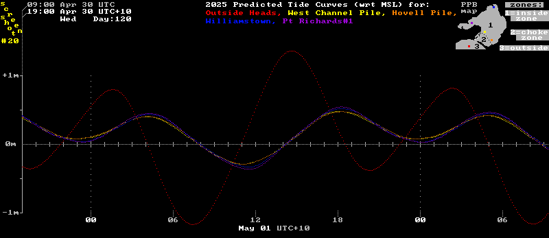
Points to note from this image for the tides on May 01 are:-
1) There is a strong height inequality between the two outside high tides and the two low tides. (Moon's declination near its peak of 27 N, and the Sun is also well north of the equator in May.)
2) The highs and lows of the "inside" tides are delayed by roughly 3 hours behind the highs and lows of the "outside" tide in the nearby Bass Strait waters.
3) During this delay period the "outside" and "inside" levels are moving oppositely to one another with both approaching a common level as the curves cross-over one another.
4) The tidal range "inside" the Bay is around 30% of the "outside" range. (But that percentage may reach up to 60% for very weak tides with low frictional losses.)
5) Around the extremes of high or low "outside" tides, there can be over a metre of difference between the "outside" and "inside" water levels. This level difference produces a corresponding difference in water pressures between any "outside" and "inside" points in the same horizontal plane. This sideways pressure differential, acting all the way down through the water column, provides the horizontal driving force that pushes water flows back and forth across the "choke zone".
6) Where the four "inside" tide curves are rising or falling strongly and steadily, there is very little height difference between them and often the different colours over-plot one another. This indicates that the slow steady currents (~0.3 knots) in the main body zone suffer very little frictional resistance.
7) Around their high and low tide times, the dark blue (far north) and the purple (far west) tide curves do show a discernible height separation from the yellow and orange curves from the southern edge of the "inside" zone. This small reverse level difference over the main body zone provides some of the dynamic force needed to decelerate, halt, and then reverse the tidal flow in the northern waters.
In the image below the dark blue and purple plots have been removed to reduce the distracting colour over-plotting. This leaves only the near-identical yellow and orange plots to show tide levels just north of the border between the "choke zone" and the "main body" zones. Two of the "choke zone's" tide curves have then been added in. These are for the Heads at Point Lonsdale (green) and for Queenscliff (light blue). Finally, vertical time lines (in orange) have been added to mark the predicted slack water times as published by the BoM.
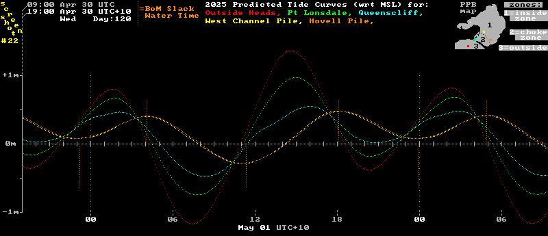
Note the vertical orange "slack water markers" are drawn above the 0m line when the flow reversal is from Flood to Ebb, and below the line for reversals from Ebb to Flood.
Points to note from this image are:-
1) The extra green and light blue curves show that where the largest outside-to-inside level difference occurs, it is distributed roughly evenly over these three regions: the "Rip Bank" area just outside the Heads, the Pt Lonsdale to Queenscliff area, and from Queenscliff to the northeastern edge of "The Great Sands".
2) During the 24 hours of 01/05/2025, there are four separate times where the tide curves converge and meet each other almost at a single point. These points mark four "Equal Levels" moments, when the sea level is essentially all at the same height from the Bay's central basin right out through the Heads and into Bass Strait. There is NO level difference (and NO "driving force") across the "choke zone" at these times. These also mark the times when the sea surface slope across the "choke zone" reverses its gradient from "downhill" to "uphill" in terms of the current flow direction.
3) The common "simple story" of Port Phillip's tides, unfortunately in very wide circulation, claims that the direction of tidal flow reverses at the "Equal Levels" point, but these plots show otherwise. Firstly in respect of events following 12:00 hours, the average rise rate of the yellow, orange and suppressed blue and purple tide curves gives a good guide to the rate at which water is accumulating in the very large main body zone. This in turn gives a good guide to the speed of inflow through the Heads because the main body zone represents about 85% of the Bay's surface area.
The maximum rate of rise here is close to +17 cm/hr at 14:30. This corresponds to a +5 knot inflowing current through the Heads according to the BoM predictions. At the "Equal Levels" moment around 17:20, the average rise rate in the main body zone is still positive at +7 cm/hr. This indicates the current through the Heads is still inward, and at a rate of around +7/17 * 5 = +2.1 knots.
That figure is a slight overestimate because it also includes some water flow coming into the main body zone just from level falls over the "choke zone", rather than from true inflow through the Heads. The excess can be estimated by using fall rates and areas across the "choke zone". That correction reduces the Heads inflow rate to about +1.9 knots at this particular "Equal Levels" moment.
It is the forward momentum of the flow at the "Equal Levels" time that allows the flow to continue forward even in the absence of any forward driving force. Since there is over a billion tonnes of water, moving at a "Heads equivalent speed" of around 2 knots, it is a formidable beast to try and halt. Frictional drag is not up to that task. At this point the gradients of the four main body tide curves continue to show reducing slopes, indicating that the inflow rate is slowing. Some of that deceleration is due to frictional drag, but increasingly it is due to the growing Reverse Level Difference as the falling "outside" level (red) drops further and further below the still rising "inside" level (yellow/orange). This creates a reverse force across the "choke zone" directed against the still inflowing current.
This Reverse Level Difference reaches around 40 cm before it is sufficient to completely halt the inflow by the time the BoM orange "slack water marker" is reached (@ 18:09). This is approximately 40 minutes beyond the "Equal Levels" moment and it indicates the residual forward stream momentum allowed the now up-slope flow to continue forward for this extra period of time before that forward momentum was fully depleted.
In the case of the two weakening ebb streams, the up-slope flow times are a little longer at over 60 minutes. The Reverse Level Differences are a little smaller in these cases. The details of the up-slope flow phase at the end of a Port Phillip tidal stream depend on several factors including; the residual amount of forward momentum that existed at each "Equal Levels" moment, and the rate at which the "outside" to "inside" level difference is then rising or falling.
The image below includes an additional curve, plotted below the tide curves. This "Bay Water Volume" curve (in mid-grey) is formed by dividing the Bay into segments where the surface area of each segment can be calculated, and where the tidal curve for each segment is well known or can be reasonably estimated. The product of tide height (in metres) times segment area (in square kilometres) gives the water volume of water in that segment (in gigaLitres) relative to its volume at the mean sea level height. All segment water volumes are added together to give a Bay wide water volume figure ( wrt MSL) over each 6 minute data interval.
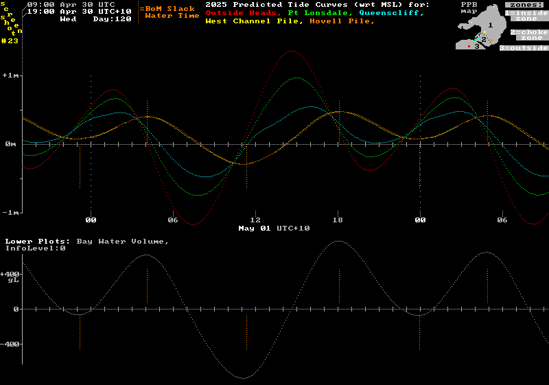
Points to note from this image are:-
1) The maximum and minimum times of the water volume curve (midgrey) match closely with the BoM's slack water times.
2) If, just before each "Equal Levels" moment, the water volume curve is rising (or falling), it will continue to move in that same way for a while after that time. This again shows the inflow or outflow does not reverse at the "Equal Levels" moments, but at a considerably later time.
The image below is further enhanced by including a Heads current curve (light blue) in the lower plotting space. These current values were determined by dividing the slope of the water volume curve (in m3/hr) by an estimate of the underwater cross-section at the Heads (in m2). This Heads current speed in m/hr is then converted into knots (kn) for plotting.
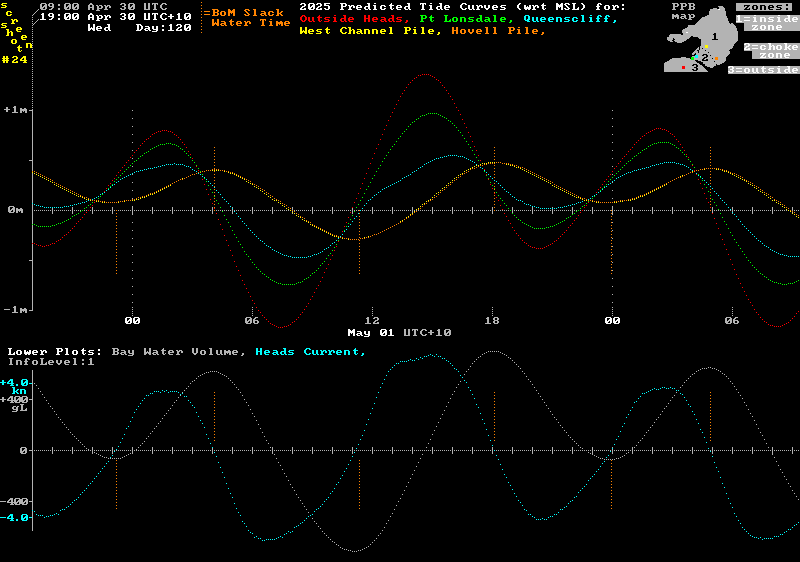
Points to note from this image are:-
1) When the light blue current curve in the lower panel, derived from the "Water Volume Modelling Method", crosses the zero current level, those times agree fairly well with the vertical orange predicted slack water time lines from the BoM.
2) Note that the current strength vs time profile around each slack water event is roughly linear in shape and passes through the zero current point at quite a steep angle. So although the currents around the slack water times are small, they are in fact changing their speed more quickly than at most other points in the tidal cycle.
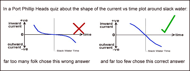
3) The main objection to the promotion of the common "simple story", which claims no level difference exists at slack water, is that it implies (and many of its followers assume) that the entrance current does not change quickly around slack water time (because with low force levels you can't change the speed of a large water mass quickly). The untrue statements that lead to this false perception are both unhelpful and potentially dangerous.
The results of a 2023 quiz about the current-time profile covering an hour or so on each side of slack water showed that less than 15% of respondents identified the correct answer. I believe the well entrenched "simple story" bears some responsibility for this disappointing result. Something a bit more truthful that promotes the correct current vs time profile would better serve boating safety. This image shows the most chosen answer on the left (wrong), and the far less popular correct answer on the right. Those selecting the correct answer included a ships Pilot, the Pilot boat coxswain, just one scuba diver, and several very experienced Port Phillip based yacht skippers who frequently venture out into the Bass Strait cruising grounds.
The image below is further altered by removing the water volume curve and then adding a level difference curve (in cm), defined as the ["outside" level (red) minus the West Channel Pile "inside" level (yellow)]. This level difference, or "driving force curve" shows in green when the current is flowing in the down-slope phase, and shows in red during the up-slope flow phase approaching slack water.
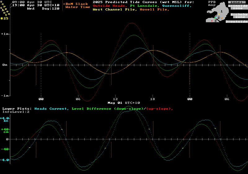
Note also that the small yellow strokes across the light blue Heads current curve mark the current strength at the "Equal Levels" times.
Points to note from this image are:-
1) The collection of yellow strokes indicate that at the time the "outside" and "inside" levels are equal to each other, the Heads current is still flowing forward at around 1.5 to 2 knots. (Well above the "zero" speed value as claimed in the "simple story".)
2) The light blue Heads current curve typically crosses the horizontal axis (zero current) some 40 to 70 minutes after the level difference curve does (green turning to red). The red section of that curve shows the period during which the level difference force is in the opposite direction to the current flow. This red colouring marks the up-slope phase where the current is finally brought to a halt, but only after its residual forward momentum present at the "Equal Levels" time has been fully dissipated by the combination of shrinking frictional drag and a growing Reverse Level Difference.
3) The short horizontal yellow strokes mark the current speed that exists at the time the forward driving force had dropped to zero. This speed is a sizeable fraction of the maximum speed achieved some hours earlier. This fraction is generally larger in the case of the weaker tidal streams. This is firstly because their rate of energy loss due to friction is smaller due to their lower speeds (flow friction rises as the square of the current speed). Secondly, these weaker streams spend less time between their maximum speed point and the "Equal Levels" point and so lose a smaller percentage of their kinetic energy between those times.
The purpose of this section is to illustrate the effects of the dynamic forces that are involved in high-mass tidal waterways like Port Phillip. Ignoring such forces, as is commonly done in the "simply story" treatments of Tides in Port Phillip, produces a significantly distorted understanding of the actual tidal behaviour. This is particularly so around the slack water times that many smaller recreational vessels will want to factor into their planning when approaching Port Phillip Heads.
A dynamic force is that component of the total applied force whose only function is to change the velocity of any mass within the system. The dynamic force "F" required to change the speed of an object of mass "m" at a rate of acceleration "a" is given by F = m times a.
This is one form of Sir Isaac Newton's Second Law of Motion. If the mass is in units of kilograms, and the acceleration (rate of speed change) is given in units of metres per second per second, then the required force will be calculated in "Newtons". An applied force of 1 Newton is required to accelerate a 1 Kg mass at exactly 1 m/s/s in the direction of the force.
While that 1 Kg mass is accelerating at 1 m/s/s, its surrounding environment must be imparting a 1 Newton net force on the mass. Conversely, at some later time when that mass has already gained some velocity and its environment changes in such a way as to decelerate the mass at 1 m/s/s, then the decelerating 1 Kg mass can be thought of as effectively imparting a force of 1 Newton on its surrounding environment.
The effective force "liberated" by a decelerating body can be thought of as then being available to overcome other opposing forces. Examples of this might include a golf ball which after being very quickly accelerated to a high speed by a mighty whack from a golf club, then slowly decelerates during the rest of its flight. It overcomes the forces of both air friction and gravity by using the reduction in its momentum to do so.
Another example, slightly more closely aligned to tidal streams, would be a child on a swing. During the downward arc of the swing, the momentum of the swing and its occupant is increased as their combined mass is accelerated along its arc by a gravity force component that acts along the arc when the swing is angled away from the vertical.
At the instant the swing becomes vertical, the horizontal force component due to gravity disappears, leaving only small retarding forces due to friction in the bearings and a little air friction. However by this time the system has acquired considerable forward momentum. This is analogous to a tidal stream having gained speed during a down-slope run, and is then able to move forward through its "Equal Levels" or "zero force" moment.
During the following up-slope phase the swing gradually encounters the additional and increasing retarding force due to gravity. These forces are overcome by continually sacrificing it's momentum as it climbs and slows during the up-slope phase. Once that forward momentum is completely exhausted, the swing briefly stops (equivalent to slack water), before reversing its motion as the up-slope phase ends and a new reversed down-slope phase begins.
Due to low air friction and low bearing friction, the swing height reached at the reversal point may be 80% to 90% of the height at the start of the previous down-swing. Water friction effects are very much greater than in air, but so too is the momentum level of the very large moving water mass of a tidal stream. The interplay of these two factors determines the ratio of up-slope to down-slope heights achieved by the time the motion briefly halts at slack water time. In Port Phillip tidal streams, this height ratio is found to be between 30% and 60% depending on the sequence of tide cycles.
The image below is a magnified and modified part of the lower plots of the previous image, plus extra markings to illustrate the dynamic force effects in Port Phillip's tidal streams.
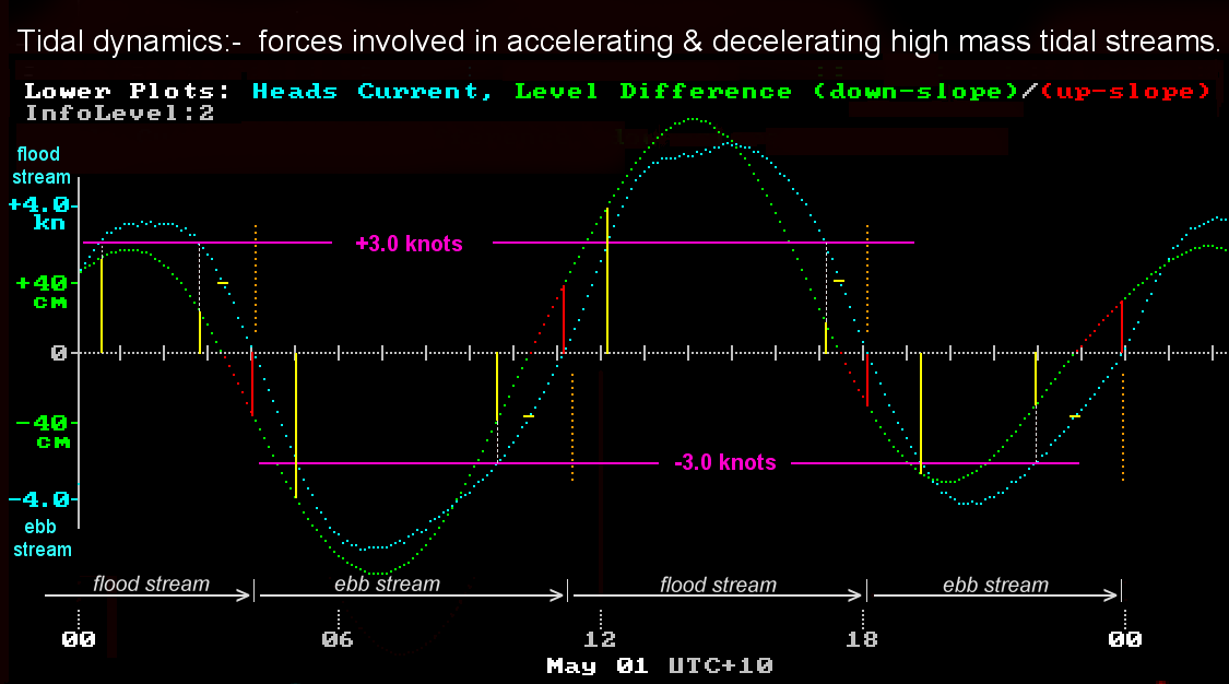
The horizontal pink lines mark Heads current levels of +3 and -3 knots. In each of the tidal streams shown, the Heads current curve (light blue) passes through one of these speed lines twice during the roughly 6 hour run of that tidal stream. One of these is while the current is accelerating and gaining speed and the other is some time later while the current is decelerating and losing speed.
Where the current crosses either of the pink 3 knot lines, a vertical yellow line is drawn from the horizontal axis to the green level difference curve. This indicates the "driving force" that was applied across the "choke zone" at that time. The red vertical lines are drawn from where the current curve crosses the zero current axis to the "drive curve" value at that time. This shows the extent to which the Reverse Level Difference grows during the up-slope phase until it is large enough to stop the forward flow to produce a brief slack water moment. It is then ready to reverse the flow direction of the tidal stream.
Points to note from this image are:-
1) Since frictional forces disappear when the water speed is zero, the red line lengths at slack water time represent just the dynamic force component needed to produce the deceleration of the tidal stream at the rate given by the slope of the current curve at those slack water times. This can also be used as a "yardstick" to estimate the dynamic forces in play at other nearby points on the curve with different rates of speed change.
2) The shape of the light blue Heads current vs time curve has some important lessons for recreational boaters who have previously accepted the "simple story" as their guidance to the shape of the current-time profile around slack water time. That story encourages the thinking that around slack water there is a pool of virtually stationary water with no driving forces in play. It is supposedly just "lolling about" waiting for a reverse level difference to develop before the water can begin moving off in the reversed direction. The curves above, along with a lot of corroborating data from other sources show this commonly believed view is wrong.
When afloat at the Heads, that incorrect story may sometimes "feel" true, but this is largely a product of how difficult it is for humans to accurately "eyeball" low strength currents. Even the common types of GPS systems will struggle to give sensible readings when drifting in currents of less than 1 knot. However using the proper equipment, thousands of measurements confirm that the speed changes at a roughly steady rate for almost an hour on either side of the slack water moment.
This occurs because approaching slack water a Reverse Level Difference steadily builds up as shown by the red dots in the level difference plot. During this time the friction drag forces that are trying to retard the tidal stream are decreasing. The combination of the decreasing friction and the increasing reverse level difference force yields a roughly steady slowing force and means a roughly steady loss of speed.
In contrast to the incorrect "simple story", the plots show that once the flow halts at the end of a tidal stream, the Reverse Level Difference that has built up instantly becomes a forward level difference for the newly reversed stream. It therefore accelerates away at pretty much the same rate as its previous deceleration. Thus the speed curve has almost the same gradient before, during, and after the zero speed moment. Knowing this number for each different slack water event would seem to be a helpful knowledge for planning activities at or near Port Phillip Heads.
On days of large tidal range, water at the Heads may go from a standing start of zero knots at slack water to reach 3 to 4 knots within the first hour. These rates of change are more usefully expressed as 0.50 to 0.66 knots per 10 minutes. This makes mental arithmetic in the boat somewhat easier. Mid-range tides usually have reversal rates in the band 0.30 to 0.50 knots/10mins. The very low range tides can have reversal rates as low as 0.15 kn/10mins.
3) During each tidal stream, when the Heads current passes through a pink line for the first time (ie. the stream is accelerating), the length of the yellow "driving force" line is considerably bigger than for the second crossing where the current is decelerating back through the 3 knot line. At the first crossing the driving force not only has to overcome the flow resistance at 3 knots, but what's left over supplies the dynamic force necessary to keep accelerating the massive tidal stream to a higher speed.
At the second crossing of the 3 knot line the water mass in the tidal stream is decelerating, and in effect using its negative dynamic force to help in overcoming some of the flow friction. This means a much lower driving force level is needed as the flow decelerates through the 3 knot line. The difference between the two drive force levels at the same 3 knots of speed is particularly noticeable in the second flood stream of the day (from 1100hrs to 1800hrs).
This is because in this case the higher "outside" tide is driving the system harder, meaning that once the 3 knot flow resistance is overcome there is a higher remaining force to be devoted to accelerating the stream more quickly than in the first flood stream. The dynamic forces in play at these times are closer to the magnitude of the stream's 3 knot flow resistance. Indeed some time after the second 3 knot line crossing we reach the "Equal Levels", or "no drive", point where all of the dynamic force released by the decelerating stream provides all the force needed to overcome the flow resistance at these slightly lower speeds of typically between 1 and 2 knots.
At first sight it might be tempting to average the two 3 knot drive levels in order to estimate the 3 knot flow resistance, but this won't yield an accurate result. Firstly this is because the +ve and -ve dynamic forces at the 3 knot level have different magnitudes because the rates of speed change are different. Secondly over the interval between the two 3 knot crossings a significant amount of water has entered or left the Bay and so significantly altered the water depths across the shallow "Great Sands" region and the reefs around the entrance. This will alter the overall flow resistance measured across the "choke zone".
By looking across all 2025 tidal streams, it is possible to plot a graph of the maximum Heads current speed reached for each tidal stream and the Level Difference of the "outside" zone with respect to the level of the "inside" zone. Since at these select times the tidal stream is neither gaining nor loosing speed, there are no dynamic forces involved. This data should be a good representation of how the frictional drag force varies with current speed:-
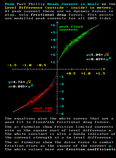
Points to note from this image are:-
0) The level difference is here expressed in metres rather than centimetres as in the previous graphs.
1) The green plot points in the upper right side of the image show, for each different inflow cycle in 2025, what the maximum predicted Heads current speed is and how much higher the "outside" level is above the "inside" level at that point. The red plot points in the lower left of the image show, for each different ebb stream, the maximum predicted outflow speed, and how far the "outside" level is below the "inside" level at that point.
2) Since there are no dynamic (speed changing) forces involved at these times, the level difference number at a particular current level is producing a forward driving force that just counterbalances the frictional drag forces experienced at those same current levels. Since the level differences produce a forward driving force that just matches the opposing frictional drag forces, we may alternatively interpret the level difference values as frictional drag levels. By combining the results from over 1,400 different flood an ebb streams during the whole year, we build up a picture of the steady current frictional drag behaviour over a large range of current strengths and level differences. These frictional drag values are the combined result of various friction related effects such as; bottom friction due to different speed layers within the boundary layers over sand and reef sea-floors, turbulence and surface whirlpool production common in fast flood streams, and wave making resistances characteristic of ebb streams exiting the Heads.
3) The two white half-parabolic curves best fitted to the data have their formulae as shown. Here each of the Heads current ("y") and the level difference ("x") variables is expressed in terms of the other, with the multiplying proportionality constants chosen to best fit the data. The upper "y=" form on each side show that the maximum current speed rises as the square root of the level difference, and that for a level difference of 1.0m across the "choke zone", the (average) Heads current over the underwater entrance cross-section is a little over five knots for a flood stream, and a bit under that figure for an ebb stream.
4) It is noted that when a flood stream reaches its maximum speed, the tide level at the Heads is near its maximum, allowing extra water to flow across the large submerged reef platforms at Point Lonsdale and Point Nepean. In contrast at maximum ebb flow times these reef platforms sit well above the waterline and so that extra flow is cut off. Similarly the depth differential across reefs just inside the Heads also adds to the slight asymmetry in the tidal flows.
While it might be thought water levels across the shallow "Great Sands" area would have a large effect at this time, this is not the case. Due to the 3 hour tide delay for that region, high or low tide at the entrance corresponds to mid-tide times over the Great Sands, with levels fairly similar for both the flood and ebb streams.
5) Notwithstanding the point 4) comments, water levels at any point in a tide cycle are also influenced by what transpired in the previous few tide cycles. For example a strong flood stream may bring 1,200+ gigalitres of water into Port Phillip but then a smallish following ebb stream may remove only 500 gigalitres of that water. This leaves elevated water levels for the start of the following flood stream, meaning that the absolute tide levels at the Heads, and the "mid-tide" levels across the Great Sands, can be quite variable depending on what happened previously. This is particularly so at times during a lunar month when a strong diurnal inequality exists. It is thought that these effects are responsible for the level difference variations seen across different plot points at the same current level.
6) The "x=" (or frictional drag) equation forms show that to drive a "y=1 knot" Heads current, the "x" level difference values across the "choke zone" are very small at just 0.039m to 0.045m, indicating very low friction levels at this one knot current strength. However as the Heads current rises to 5 knots, the level difference values increase 25 times to 0.98m and 1.13m to provide the necessary drive force.
Looking at these results the other way around, the dramatic reduction in frictional drag as the current speed decreases to low values makes it clear that the common "simple story" of Port Phillip's tides, which claims its massive tidal streams are brought to a halt by frictional drag forces alone, is virtually impossible. Another retarding force must be involved, and a growing Reverse Level Difference retarding force fills that bill perfectly.
7) The plot points in the previous image have a "gap" in the low current region between +1.5 knots and -1.5 knots. This is because there are no weak tidal streams with peak speeds below these limits. (A single BoM flood max prediction of 0.96 knots on 28/01/2025 can be dismissed as an error in the algorithm as it's value falls well below the usual relationship of around 3.3 cm/hr of main body height rise rate per knot of inward entrance current.) Further work with weak streams, incorporating the necessary corrections for stream speed changes, supports the given drag equations down to current speeds below 1 knot.
8) Vessel owners should be familiar with the rapid reduction in frictional drag as a drifting vessel is slowed down by skin friction alone (ie, no use of engine thrust). The effect depends on the ratio of the vessel's forward momentum to the skin friction of the hull moving through the water. Suppose this ratio is such that a large vessel moving at speed and then disengaging the engine at 8 knots, takes just 1 minute to slow to 4 knots while "coasting along" and using only the drag forces to slow the vessel. It will then take an additional 2 minutes to halve the speed again from 4 knots to 2 knots. An extra 4 more minutes are needed to halve the speed again from 2 knots to 1 knot, and an additional 8 minutes to slow from 1 knot to 0.5 knots, etc. A quarter of an hour has passed and we haven't come to a complete halt yet! So while frictional drag can be relied on to "apply the brakes" at the higher speeds, it rapidly becomes ineffective as the speed drops off.
9) With a reasonable confidence in the frictional drag equations, it then becomes possible to follow selected ebb and flood stream cycles over their full run and then separate out the friction and dynamic force components from the total applied force that controls the growth and decay of of currents in the tidal stream. Here are three typical examples:-
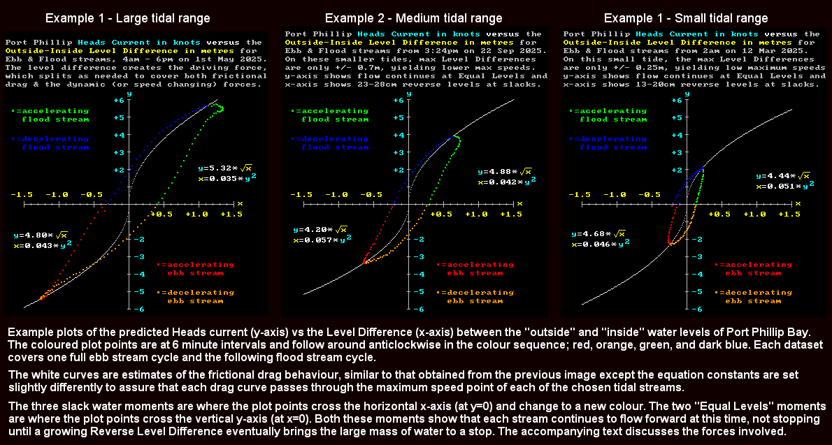
Consider the acceleration phase of a flood stream (green) in any of the examples shown above. The horizontal distance from the y-axis to a green plot point represents the total inward force applied across the "choke zone" at that particular moment by the fact that the "outside" level is above the "inside" level. This force is initially much larger than the corresponding frictional drag force represented by the distance from the y-axis to the white curve. The excess of "drive over drag" (ie. the horizontal distance from the white curve to the plot point) is the dynamic force responsible for accelerating the flow to a higher speed as evidenced by the upward green curve. The vertical separation between the 6 minute plot points indicates how rapidly the speed of the current is changing. This spacing can be seen to decrease in either "lower dynamic force" cases (eg. from Ex1 to Ex3), or for "higher friction" situations (eg. currents > 3 knots).
Note in examples 1 and 2 that the green curves display a slight "nose shape" around the maximum level difference values and the current continues to increase slightly as the level difference begins to decrease below its maximum (x) value. This indicates that for large "outside" tides, the flood streams don't get the chance to reach their terminal speed ("drive" = "drag") until some time after the "drive" level begins declining. That time delay looks to be around 50 minutes (by dot interval count). This is just a delay due to the large mass being accelerated. It is the mirror of the momentum delay met before during deceleration where the stream only reaches zero speed well after the drive level reaches zero.
At the maximum speed point the "drive" and opposing "drag" forces are in momentary balance, but then the strength of the "drive" force decreases to becomes less than the "drag" force. This excess of "drag" over "drive" means the stream starts its deceleration phase. The dynamic force ("drive" minus "drag") then becomes a negative quantity and so the speed and momentum of the tidal stream decreases. As the Level Difference, current speed, and drag force all decrease (dark blue), we reach a point in high mass streams where the Level Difference reaches zero but the current speed has not.
At this "Equal Levels" moment, the tidal stream is just coasting along without any external applied force. It is however being decelerated by its own frictional drag force. Beyond this point a Reverse Level Difference grows and its increasing force is in the opposite direction to the water flow. Together with the decreasing drag force, also in the opposite direction to the water flow, this combination aids the slowing of the stream at a roughly uniform rate. Eventually this increasingly uphill flow serves to dissipate all the forward momentum of the water mass and the forward flow ceases. The slope left in the water surface at this slack water time provides the force to accelerate the water mass in the reverse direction, again at roughly a uniform rate.
The evolution of the ebb stream (red & orange) follows a similar story except that at very strong ebb current speeds there is an absence of any "nose" like feature. This is because the higher friction coefficients mean that at the time of peak driving force for an ebb stream, it is much closer to its terminal speed than is the case for fast flood streams. The crossing over of the orange and white curves seems to indicate that the white parabolic drag curve might not accurately reflect the full friction story. A feature of strong ebb flows is the tendency to form a rather narrow "jet" of outgoing water outside the Heads that continues to be felt several miles out to sea. This jet also is characterised by large breaking waves which may mean the resistance plot might have a different shape at high ebb stream speeds. Almost all the work behind these webpages has been about the low current times around the Equal Levels and Slack Water times, with very little attention paid to the very high current phases. These are also more difficult and less safe to verify through direct measurements on the water.
Dynamic forces are significant in Port Phillip, and to ignore them completely as the "simple story" will not give an accurate picture of what really goes on at and near Port Phillip Heads. The "simple story" appears to confuse "driving force strength" with "water speed", whereas the Laws of Motion are clear that a force only dictates the rate of change of speed, and the mass of the object is also involved. The "simple story" also asserts that after a tidal stream reaches its maximum speed, it will then decelerate to 0% of that speed by the time the "Equal Levels" point is reached.
The truth is that all the direct measurements and modelling work show that by the "Equal Levels" time the streams have typically slowed to just somewhere between 25% to 50% of their maximum speed. This means Port Phillip's tidal streams will always overrun the "Equal Levels" point and only stop after a sufficient Reverse Level Difference, of from 10 cm to 40 cm, has built up to finally halt the flow. This may take an additional 30 to 90 minutes of forward flow, depending on the particular tide cycle sequence.
The existence of the reverse force at slack water time results in a completely different shape for the current vs time profile around slack water time than is implied by the incorrect "simple story". It is on these safety grounds that its continued promotion by individuals, clubs, organisations, and government bodies must be discouraged.
The composite image below shows how tide curves, together with "drive" and current curves, spell out a better story of Port Phillip's Tides and Tidal Currents. The upper panel (#1) shows the relevant tide curves. These are not the curves usually published in the various forms of "Tide Tables". Instead they show heights relative to some fixed height datum common to all locations. In this case that reference datum is Mean Sea Level (MSL). Only when this is done can the height differences between the curves be accurately interpreted as the strength of the driving forces acting between those different locations.
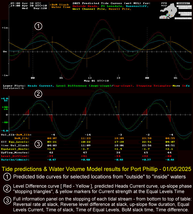
The middle panel (#2) shows the key aspects of the "driving force" and the resultant Heads current strength. It reveals the true timing of the "Equal Levels" moment, and the forward current that still exists at that point (yellow strokes). The red "Stopping Triangles" show the slow build-up of the Reverse Level Difference, and its final value, as the current overshoots the "Equal Levels" moment and continues flowing up-slope towards the actual "Slack Water" moment where the flow velocity briefly becomes zero before reversing. The white highlighted base of each "Stopping Triangle" shows the duration of the up-slope flow phase.
The different current profiles for strong flood and ebb streams discussed previously in the "three example current vs force plots" image, showed flood stream examples 1 & 2 had a "nose" while the ebb streams do not. This is illustrated again in the current vs time plots of panel #2 in the above image. All three flood (+ve) current curves show either "flattish" or "slowly rising tops" around their peak current values.
This is consistent with a system where approaching maximum driving force, there is still quite some margin between the rising applied force level and the rising frictional drag level. Due to this lag, a slow continued acceleration of the current's speed is still possible after the applied force peaks. The actual peak speed point is then attained some time after the driving force has begun its decline.
A not very close but maybe helpful analogy is that of a skydiver jumping out of a plane. The skydiver takes some time to reach their terminal velocity because the net force of (gravity - frictional drag) also has to accelerate their body mass to that high terminal velocity. Of course in the tidal stream case of a now diminishing applied force, the current never reaches the "terminal velocity" associated with its peak level of force.
In the ebb (-ve) current curves, because of their higher frictional coefficients, that margin of driving force over friction is very small or barely exists at all. So in strong ebb streams there is no broad current maximum and the peak current occurs very close to the peak drive time. Only in the weaker ebb streams do we see the peak current time occurring well after the peak drive point.
Panel #3 shows a table of various data associated with each stream reversal as produced by the Water Volume Modelling. Included in this table are the slack water time predictions as published by the BoM. In most cases the agreement is fairly good. The columns of numbers make more sense if read from the bottom upwards. The rather cryptic coloured names up the left edge of panel #2 are made a little clearer in the lowest three lines of text at the bottom of the image.
It will be apparent from the plots that the characteristics of each slack water event depend not only on the particular tide curve behaviour during the running of the previous tidal stream, but also on the tide curve behaviour after that slack water event. This is because both behaviours contribute to the shape of the all important "drive curve". Given that the Bay tides also have a strong diurnal component and that this means tidal patterns don't closely repeat again for over 18 years, we see there can almost be an endless variety in the possible combinations of "before slack" and "after slack" tide curves. This leads to a wide scope of behaviours as the tidal streams reverse around slack water time. Some different examples are given in the image below and show the wide shape variations possible for the Heads current plots, the level difference plots, and the all important red "stopping triangles":-
The best way to show the full variations that occur during tide stream reversals is to construct histogram plots of some of the main parameters associated with each slack water event over a full years worth of tide cycles. A histogram plot counts the number of times in the year a particular parameter value occurs as a vertical column, with the actual parameter values being plotted along the horizontal axis. The six coloured histogram plots below are from Port Phillip water volume modelling. They show the distribution of count values for six different slack water related parameters over all 2025 tide cycle predictions.
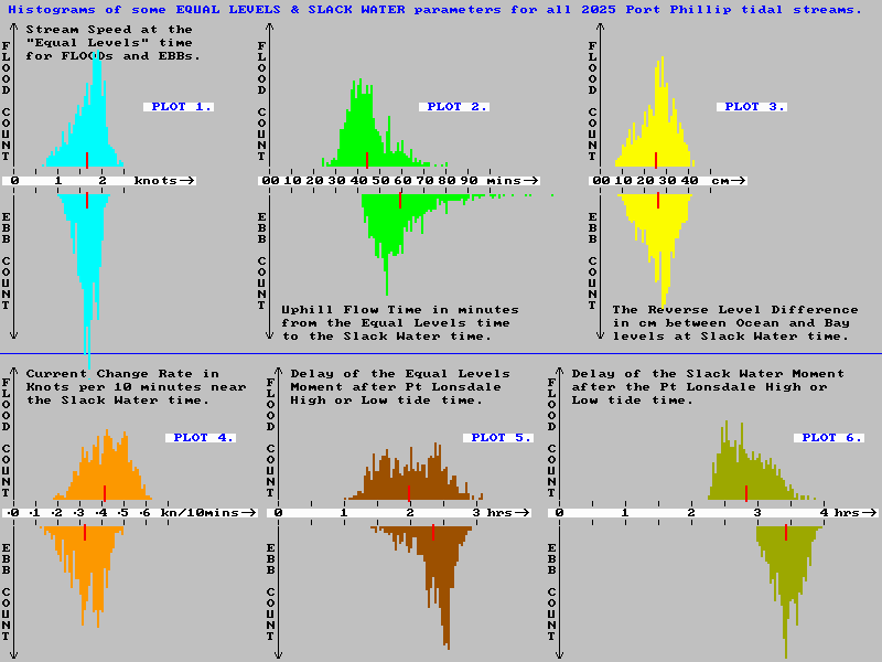
Plot 1. A typical tidal stream through Port Phillip Heads may bring in or remove around a billion tonnes of seawater, moving at speeds of up to 10 kph. There is an enormous level of inward or outward momentum added or removed from the Bay's waters during the 5 to 7 hour run of the tide. (momentum = mass by velocity).
At the same time this process is occurring, some of that momentum is removed by frictional loses, which increase rapidly at the higher entrance current speeds. The tidal streams also "push" or "pull" at the large water mass located in the main body zone and so force it into motion. Thus a significant part of the entrance current's momentum is shifted into the main body zone. Due to the Bay's wide and moderately deep central basin, the currents here are much slower, so frictional losses there are very small and the momentum is effectively "stored" in these waters to be removed later in the up-slope phase.
As the tidal streams slow towards the end of their run a key question is how much residual momentum remains within the system at the "Equal Levels" point where the stream's forward driving force ceases. That momentum number is what allows the tidal stream to continue flowing beyond the "Equal Levels" time, and also determines how much needs to be dissipated before the stream is finally brought to a halt to give "Slack Water".
The Plot 1 histogram shows the distribution of entrance current speeds that remain at the "Equal Levels" time for all 2025 flood and ebb streams. The red markers show the average speed value for the flood and ebb distributions. These are very similar at around 1.65 knots. The speed of the tidal stream at the Equal Levels moment is a measure of the amount of forward momentum that remains in the Bay's waters.
Scientifically speaking the true measure of that residual momentum is equal to the total mass of water in the Bay (about 25 billion tonnes) times the velocity of its Centre of Mass. That will be some point near the middle of the Bay, with a velocity roughly 1/20th of the velocity of the entrance current. In rough terms that is 25 billion tonnes times 0.08 knots worth of momentum that has to be dissipated before the flow can come to a halt.
It can be hard to get a proper perspective on a very large number multiplied by a very small number. If we think of a fully loaded 300,000 tonne supertanker moving at 20 knots, we have something for comparison. The forward momentum in that supertanker would be equivalent to 300,000 * 20/0.08 = 75,000,000 tonnes of mass moving at 0.08 knots. So the Bay's forward tidal stream momentum at the Equal Levels time is roughly equivalent to:-
(25,000,000,000 * 0.08) / (75,000,000 * 0.08) = 333 fully loaded supertankers all steaming at 20 knots. We can imagine that enormous supertanker fleet will take quite some effort to stop!
The only way to produce a reversing force of the magnitude required is the "hands off" approach of simply allowing the stream to continue to flow into an increasing up-hill slope across the "choke zone" as the "outside" and "inside" levels are now moving apart. This is a little like when road engineers sometimes provide an uphill sloping "off-ramp" at the site of a downhill hairpin bend. This allows trucks with a brake failure to take the off-ramp and slowly bring their vehicle to a halt without loss of life. Of course it takes some time for the up-slope run to exhaust all the forward momentum.
Plot 2. This histogram shows the distribution of up-slope flow times for all 2025 flood and ebb streams. We immediately see the distribution of the up-slope flow times for ebb streams is skewed towards longer times and has a very long tail. Although the average time as shown by the red mark is around 60 minutes, on a few rare occasions it extends to around double this. In contrast the average for a flood stream is to run for only 44 minutes beyond the "Equal Levels" time.
Since the average stream speed at the "Equal Levels" time is almost the same for floods and ebbs, and that the total mass of water in the Bay remains about the same, the residual momentum levels should also be very similar. Why are the two up-slope flow time distributions so different?
The answer here is that the rates at which that momentum is removed is different for flood and ebb streams, resulting in different times to complete the job of stopping the flow. A key factor in determining the rate at which residual momentum is "burned off" is the rate at which the Reverse Level Difference grows. In turn around 90% of that growth rate is determined by the rise or fall rate of the "outside" tide just before the slack water time. The image below shows the distributions over all 2025 tides of the "outside" tide's rise or fall rate near slack water time:-
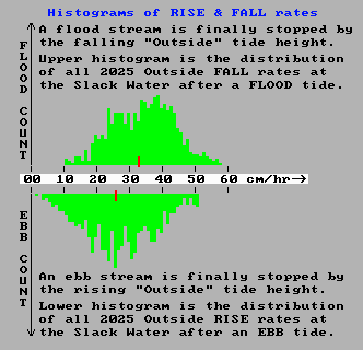
Because of the complicated way the tide slops into Bass Strait from both ends, each of which has large islands partly blocking those entrances, the rise and fall rates of the tides are not symmetrical outside Port Phillip Heads. There is a significant skew as shown by the two histograms. On average at slack water time after a flood stream, the "outside" tide height is falling at around 33 cm/hr, or 0.55 cm/minute. In contrast, on average at the end of an ebb stream the "outside" tide rises less strongly at only 26 cm/hr (or 0.43 cm/minute). The different rates at which "the brakes are applied" near the end of each stream type results in a time skew in the up-slope flow times as shown in Plot 2 of the previous image.
Also of note is that the rise rate histogram for stopping ebb streams shows quite a number of very weak tide cycles that have exceptionally weak "outside" rise rates of less than 10 cm/hr. These situations mean the build up of the "stopping triangle" is very slow, resulting in the long tail of the up-slope flow times (90 minutes plus) as shown for ebb streams in Plot 2 of the earlier image.
Most of these events are related to when the Moon's declination is near its extremes, producing a very strong diurnal inequality in low tide heights. In the most extreme case on Feb 26 - the left most data point in the plot above, the low "outside" tide was only 22 cm below the following high tide. The corresponding "inside" tide range was only 15 cm, with only a 300 gigalitre Bay water volume change compared to figures from 500 gL to 1,500 gL for most other tides.
The resulting very slow growth of the Reverse Level Difference took more than 2 hours and 10 minutes to build up to +14 cm, just enough to finally stop this weak ebb stream. That stream was in the down-slope phase for 162 minutes and the up-slope phase for for 131 minutes. The average Heads outflow rate was around -1 knot. The long up-slope phase goes to show that with the weak friction levels at low speeds, how difficult it is to stop even low speed streams. It also brings home the point that the simple story's claim that high mass Port Phillip tidal streams can stop by the "Equal Levels" time just by using their own frictional drag begins to look rather silly.
The previously shown higher friction drag coefficients for ebb streams, together with the timing skew in the up-slope flow times histogram, indicates that on average, ebb streams run a little longer than flood streams do. This is found to be the case with the average Port Phillip outflow lasting around a little longer than the theoretical 6 hrs 12 mins, and the the average inflow lasting a little less than that figure.
Plot 3. The yellow histogram shown in the second image back from here shows the distribution of the Reverse Level Differences attained at slack water time for all flood and ebb streams in 2025. The two distributions are quite similar and the average values (marked in red) are almost the same. This is in line with the Plot1 "Speed at the Equal Levels time" histogram indicating that on average, at the "Equal Levels" time, the residual forward momentum levels in both types of streams is very similar. This requires a certain Reverse Level Difference to fully dissipate, it is really then only a mater of different growth rates in the Level Difference that determine how long it takes to achieve the required "stopping" difference.
The previous "six-pack" histogram image is repeated here for convenience of discussing the lower three plots:-
Plot 4. The orange Plot 4 shows the distribution of predicted reversing rates of the streams at all slack water times in 2025. The rates at which the speed of the Heads current changes are given in the rather pragmatic boating units of knots change in speed per 10 minutes. Hopefully this is a lot easier to get your head around rather than using the standard "scientific units" of m/s/s. Some may bristle that saying "knots per unit of time" sounds like an ignorant landlubber, but they can relax as it is a perfectly legitimate (and pragmatic) way of expressing an acceleration or deceleration rate.
The orange histogram also shows a skew in the distributions, with flood streams usually reversing through slack water somewhat more rapidly than ebb streams do. This effect is explained with reference to the earlier small histogram image of the "outside" Rise & Fall rates around slack water time. That showed asymmetry in that typically around slack water time, the "outside" tides fall faster (and so stop flood streams more quickly) than later on when they rise slower (and so stop ebb streams more slowly).
While conducting my "Slack Water Quiz" some years back, the Ship Pilot I had bailed up with my quiz question on the current vs time profile was abled to pick the correct answer within seconds. However as he walked off, he stopped, turned, and came back. He said he just wanted to check that the question referred to a reversal from flood to ebb. He then went on to say "those reverse a bit more quickly than from ebb to flood". So although the difference is not that large, his years of taking ships in and out through the Heads had enable him to "feel" the difference that I'm sure many others would be completely unaware of.
Plot 5. The upper brown Plot 5 histogram shows the distribution of the delay times between high tide at Point Lonsdale and when the "outside" tide has fallen enough to equal the "inside" level. The lower brown histogram shows the distribution of the delay times between low tide at Point Lonsdale and when the "outside" tide has risen enough to equal the "inside" level.
This time skew towards longer times for ebb streams is also mostly explained by the same asymmetry in the Rise & Fall rates of the "outside" tide. In this case those quicker fall rates mean that the lower "inside" level is reached more quickly. The slower rise rates mean the rise from low "outside" tide to the higher "inside" level takes on average about 22 minutes longer.
Plot 6. The olive coloured Plot 6 shows the distributions of the delay between high or low tide at Point Lonsdale and the following slack water time. The time skew here is due to a combination of the ebb stream's longer time (average about 22 minutes longer) to reach "Equal Levels", plus the ebb stream's longer up-slope flow time (average about 15 minutes longer) from "Equal Levels" time to "Slack Water" time.
So in summary, the slack water at the end of a flood stream occurs between 21/4 hours and 33/4 hours after High Tide at Point Lonsdale. The slack water at the end of an ebb stream occurs between 3 hours and 4 hours after Low Tide at Point Lonsdale.
There is also the issue that a certain percent of the audience will be colour blind. It is also unfortunate that a lot of these images have a very restricted colour pallette due to the old video card specification I program under. In addition those not familiar with the geography of Port Phillip may struggle putting unfamiliar place names into the right geographic context.
The challenge is to show the behaviour of tide related quantities over both geographic location and time, all on a 2D computer screen. Another approach that may be helpful to some is to concentrate more on showing tide heights across the whole Bay and out through the Heads into Bass Strait, and only show the situation at selected important times rather than at every 6 minutes. This approach concentrates on showing the small sea surface slopes that provide the forces to drive the tidal currents.
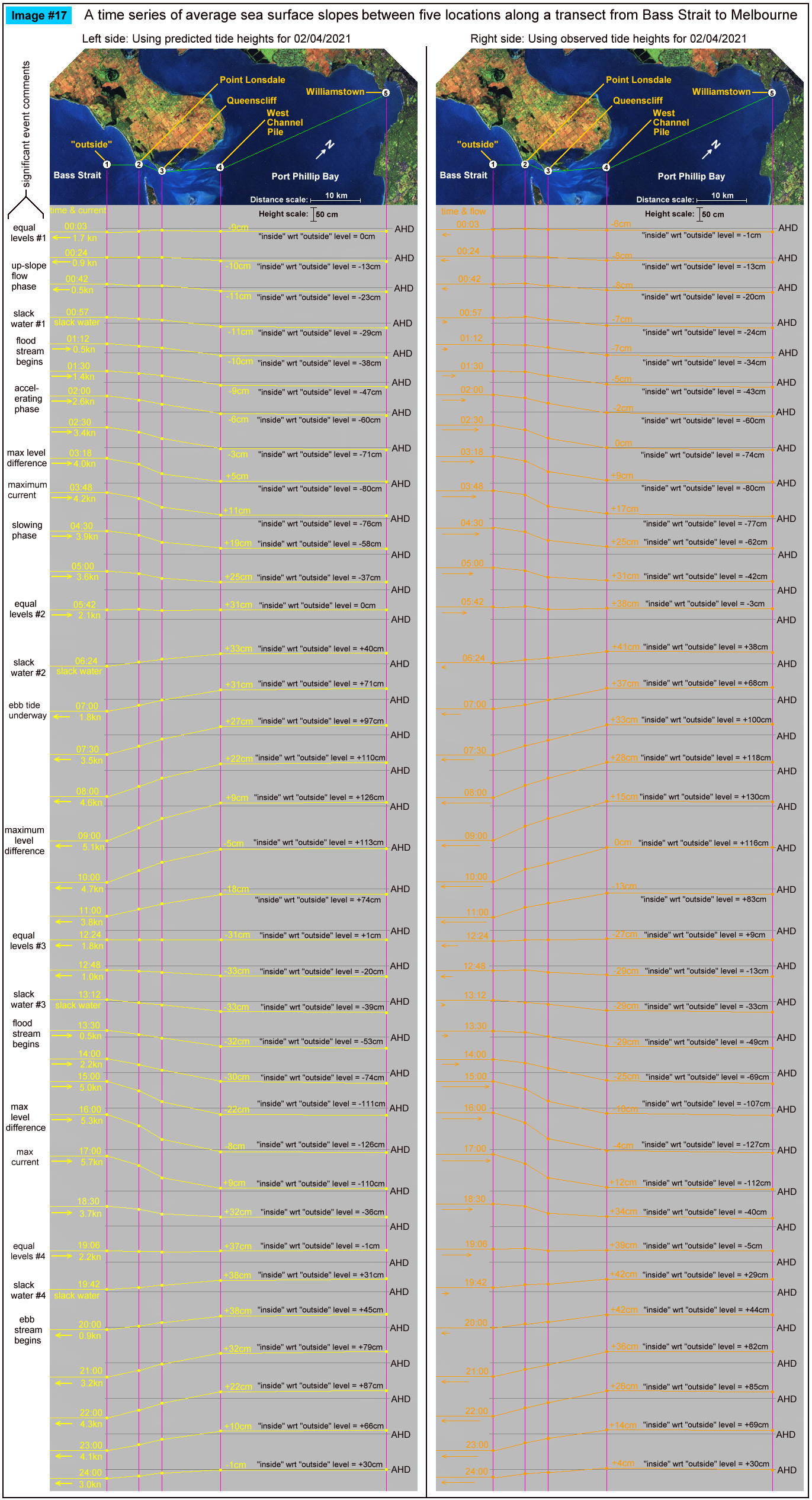
The split screen images below attempt to show the tide heights across a distance from outside the Heads all the up to Williamstown (Melbourne) along a "not quite straight" transect line (in green). Note the maps in the image have been rotated 45 degrees clockwise from the usual "North Up" orientation. This allows the most important parts of the transect, choke zone locations #2 --> #4, to be approximately horizontal across the screen.
The left hand side of the screen shows the predicted tide heights at selected locations from the Bay's tide gauge network. The right hand side of the screen shows the measured heights of the tide at those locations. All tide heights have been corrected to the Australian Height Datum (AHD) before plotting. This allows these points to be joined across the screen to represent accurate sea slopes along the transect.
The yellow and orange "joining lines" running across the screen then show for each selected time the sea surface slopes along the transect. Note however than the vertical and horizontal distance scales are vastly different. This amplifies the slight sea surface slopes between locations so they can easily be seen.
The different selected times are catered for by having different plots for different times running down the screen. At the left of each plot the time and Heads current value are shown. The current numbers come from the water volume modelling method, but when the real tides are used with this method, their slightly wobbly nature means a rolling average of three readings had to used to create a sensible current representation. These are then shown not as a number, but by a directed orange arrow whose length represents the Heads current value at that time. More details of how the current values were obtained is covered in POST #1.
The black text down the left margin of the image describes the selected event shown by that "slope plot". These plots cover a 24 hour period showing four tide stream reversals:-
Points to note in this image are:-
1) The "Equal Levels" time is a rather extraordinary event with the sea surface at essentially the same level over some 75 km.
2) At that time, and with NO driving force in existence, the entrance current is still running at around 2 knots.
3) The steepest sea surface slopes occur over the "choke zone" roughly from locations #2 to #4. These slopes show a large level difference force is needed to drive the tidal current across the "choke zone" at these times. The flow resistance across this zone is made up of a mix of frictional drag and inertia effects where the large water mass is being forced to undergo a change in speed. The frictional resistance dominates at the higher current speeds while inertial resistance effects dominate in the lower speed range.
4) The residual forward momentum still in the tidal stream at the "Equal Levels" time can drive the current flow for a further 30 to 50 minutes.
5) The current only stops, and is ready to reverse, when the Reverse Level Difference across the "choke zone" has grown to around 30 to 40 cm.
6) The orange slope lines on the right hand side from the measured tide data are generally similar to their left side counterparts except that all heights are around 4 to 6 cm above the predicted ones. This is due to slightly higher sea levels which can be brought about by a number of weather effects; lower than average air pressure creates higher levels through the inverse barometer effect, or raised levels due to a "tidal surge" event, often the aftermath of strong SW to NW winds raising levels in Bass Strait.
7) Across the "main body" of Port Phillip (eg. 4 --> 5), there are only very small surface slopes at any stage of the tide cycle as its level rises and falls.
I have used data from a low resolution hydrodynamic model of Port Phillip to create the animation below to help visualise both the sea level and tidal current behaviour. It may help to understand the large inertia and momentum effects on the current's behaviour, and the relationship of both the sea level differences and the currents to the "Equal Levels" and "Slack Water" moments.
Twin "maps" of Port Phillip are shown, with colour coded sea level heights on the left map and colour coded current speeds and direction on the right map. The lower section shows graphical plots of the "outside" (white) and "inside" (red) sea level heights. Each height is taken as the average value of a cluster of cells around the white and red locations mark with a *. The lowest plot is of the level difference (Bass_Ht - Bay_Ht). This shows as green during down-slope current flow and as red for the up-slope phase.
It is this level difference that drives the Bay's currents and tides. When one side is higher than the other, water pressure differences create a horizontal force that acts on the enormous water mass between the ocean and mid-bay regions. However this force, modified by the frictional resistance, only determines the rate of change in the water's speed and does not in itself directly determine the resulting speed, or indeed the direction of the water flow.
The level difference is a measure of the strength of the applied "driving" force. Forget the Moon and Sun, they serve only to wobble the "outside" ocean level up and down, and have no direct gravitational effect on water bodies the size of Port Phillip. Tidal streams at the entrance, and tides within Port Phillip Bay, are all the result of these level difference forces pushing a large mass of water back and forth while also overcoming various frictional resistances. These inflows and outflows alter the volume of water residing in the Bay and hence make its internal tide heights rise and fall.
The animation's blue plot shows the resulting current velocity through the Heads. Positive values indicate a flooding (inward) current. Note that the slope of this blue curve is at its steepest as it passes through the slack water times. Note that factual errors within the "simple story" lead many to believe the current profile is fairly flat around slack water time.
The yellow plot shows the variation over time of the volume of water residing within the Bay relative to its volume at Mean Sea Level (MSL). Naturally it's minimums and maximums correspond to the slack water times. The changing numerical values of each plot point are shown as coloured numbers below the maps.
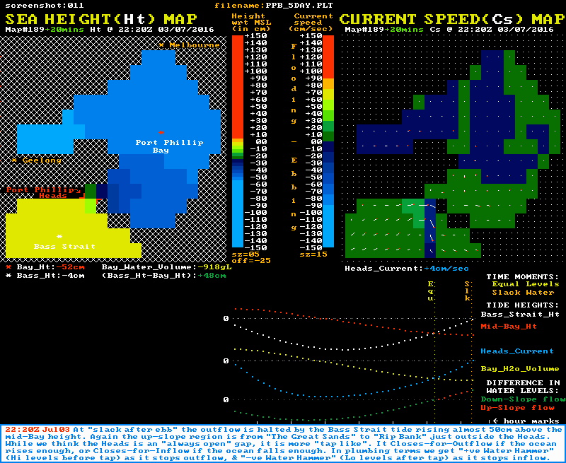
The animation shown above had its colour banding for sea height set at 15 cm per band so the whole cycle could be accommodated in the limited colour pallette available. The two static images below are of "slack after flood" and "slack after ebb" respectively, but with a finer colour banding set at just 5 cm per band. These better demonstrate the physical extent of the reverse slope regions at slack water time.
"Slack after FLOOD"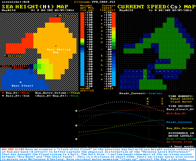
Note also that the graph section of both images shows that at the "Equal Levels" moment (yellow time line), the Heads current is still flowing with some strength. It is the residual momentum in the tidal stream at this time that powers the up-slope flow phase until slack water is reached (orange time line). Again note the speed of the current changes most rapidly around the slack water times.
There is also a static image of a sequence of eleven commented screenshots at this link: See 11 frame sequence. This may render as a tall and skinny image, in which case the image will need to be "clicked" to bring it up to full width. The commented frames can then be scrolled through one at a time at your own pace.
Similar inertia and momentum effects occur in Bass Strait itself, where significant water flows occur between the major headlands and the major islands of the Strait. It is particularly strong in Banks Strait where water flows through a 20 km wide gap between the northeast tip of Tasmania and the southernmost islands of the Furneaux group. A location map for Banks Strait is shown below.
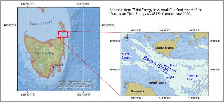
Although the maximum currents here are lower than at Port Phillip Heads, the width and depth of Banks Strait means the mass flows are far higher. This gives higher levels of water momentum that need to be dissipated to finally stop a tidal stream. The up-slope flow phase of tidal streams in Banks Strait lasts for around 2 hours, or 30% or so of their total flow time. At slack water a reverse level difference of around 70 cm exists between Tasman Sea waters at one end of the strait and the Bass Strait waters at the other. A "Sea Height & Current Speed" animation of Banks Strait is shown below:
Of note in this waterway is that the tidal current speed at the "Equal Levels" time is still more than 50% of the maximum speed. Also of note is that the shape of the blue current plot has the most rapid changes in current speed occurring near slack water. Again we see that in systems with high-mass tidal flows, any "simple model" that tries to suggest that current speed is proportional to the instantaneous level difference is counter productive in both aiding understanding, and improving boating safety.
For a number of years a CSIRO hydrodynamic modelling group have operated a nation wide hydrodynamic model of Australian waters with a number of "zoom inserts". These enable the system to produce both sea height and tidal current strength maps for those "zoom" areas. During 2023 I collaborated with the CSIRO bods behind this model to successfully lobby for adding a "Port Phillip (& Western Port)" zoom insert. That model has a higher spatial resolution than the previous images shown here. The output is static images and the two colour coded "maps" are not presented together in the one image but the user can toggle back and forth between them at will.
Other useful features, such as "mini-graphs", were then also added to help boaters better understand the tides and streams at Port Phillip Heads. The CSIRO model predicts tides and streams at selected 30, 60, and 90 minute intervals over a full year for some key tidal regions around Australia. Predictions of slack water time for Port Phillip Heads are also included but are not accurate enough to be used for any navigation decision.
The "maps" output from this model are freely available through the Australian Ocean Data Network (AODN). Those wanting to play with the new PPB zoom insert recently added to this system can start with the link that follows. This lands at a "slack after flood" event in February 2025:- PPB Levels & Currents February 2025.
Use the controls listed below to toggle back and forth between the Height and Current maps as you step forward through a time sequence that includes several maps with the words "slack at x at . . . UTC". Note that only maps with the slack water time within a few minutes of the "map time" will give an accurate portrayal of the Reverse Level Difference.
[SPD/SL] = toggles the map between current SPeeD and Sea Level mapping modes.
[NEXT] & [PREV] = steps forward or backwards in time.
To explore other dates use:-
[DATE INDEX] = allows choice of date and approximate time (note these are UTC)
To explore other selected regions of Australia use:-
[tides] = shows a map of Australia, with the available "zoom inserts". Click one to select that region
It is hoped this webpage has delivered a large serve of evidence, from a variety of sources, to encourage the many boating folk who operate in the current affected southern end of Port Phillip, and who have been influenced by the widely promoted "simple story" of its tides and currents, to turn away from that story and embrace the far more accurate "better story" presented here.
I am fully aware from feedback that for the "rusted on believers", this may be a difficult ask. This should not be seen as a burden but a joy! The "old story" I am asking you to toss overboard is full of untrue statements, has several internal contradictions, is at odds with the laws of motion, lowers your safety near the Heads, and was never supported by any robust science.
Rest assured that I am redoubling my efforts from the top government levels downwards to get the "old story" removed or revised as quickly as possible. The grounds for ditching the old "simple story" seem very straightforward; a) untrue claims are being made b) those claims lower safety, and c) it reduces your understanding of "how the Bay really works".
However, past experience has taught me that where an incorrect opinion has been held for so long it has almost become "a religion", then minds can't be changed easily. This even seems to be true when there is no evidence to support the old view and yet truckloads of evidence to support the new one. Human nature is a complex beast indeed.
To return to the Index Page of this website use this link: To Index Page
--------------------------------- The End ----------------------------------