This post introduces water flow principles using several simple "thought experiments", and then advances these into showing an animation of a functioning hydrodynamic model of the Bay and its entrance currents over several tidal cycles. This post is aimed at persuading folks that the widely believed official advice about Port Phillip's tides and currents is not entirely correct, and that their safety can be improved a little by a better understanding of the actual water flows.
The preliminary thought experiments ask you to imagine two vertical glass tubes, joined at their bottom ends by a horizontal tube containing a tap at its mid-point. The equipment looks a little like the letter "U" with the tube's upper ends open to the air. The tubes are partly filled with water. Two different "thought experiments" will be performed on water flow basics. Each requires a simple set-up routine to be done first before the experiment can begin. The set-up routine steps are described in this diagram:-
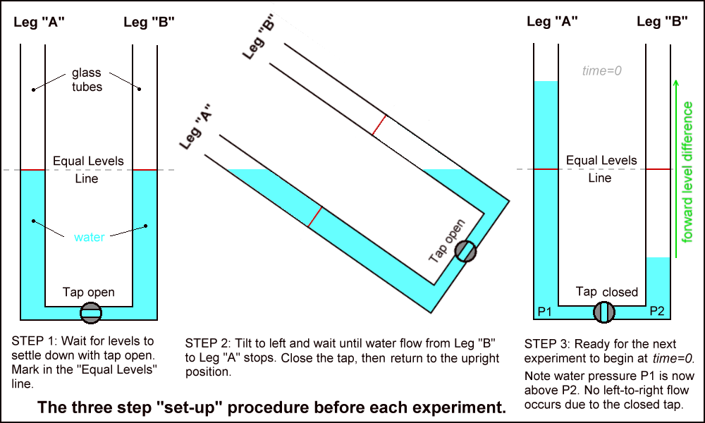
Step 3 of the sequence leaves the U-tube with tap closed and a significance difference in the water levels in the two Legs "A" and "B". That level difference (green arrow) has been called a "forward" level difference because the water pressure differential (P1 - P2) will push the water in the direction of the green arrow once the tap is opened.
Earth's gravity gives any object in its field a level of Gravitational Potential Energy that depends on its height above the centre of the Earth and the mass of that object. A part of that potential energy is released if that mass is allowed to move downward to a lower height. In STEP 3, the potential energy of the raised part of the water in Leg "A" will be released once the tap is opened and the water moves back to the "Equal Levels" condition.
Examples in the real world include hydroelectric schemes where water in a high mountain dam is allowed to flow into a lower level river while a water turbine "harvests" some of the change in the water's gravitational potential energy as it flows downward between the two levels. The process converts some of the energy released into useful electrical energy. The conversion is never 100% efficient, the main losses being to flow friction in the massive pipe network needed to implement such schemes.
On the domestic front, the local water supply system uses uses large tanks or water towers located at a high point in the suburb to store drinking water. This can then flow down through an extensive pipe network to supply water under pressure to the domestic end user.
Inside the house most of the water's potential energy is "discarded" as the end customer is really only interested in filling their sinks, baths, and basins. Most of the released energy is dissipated by flow friction, mostly as it passes through the last tap washer. This energy loss goes into a very slight heating of the water as it passes through the tap.
Outside the house the energy release is often more productive. A garden hose, as well as having frictional losses, also converts some of the potential energy into the kinetic energy of the fast moving jet of water coming out of the hose nozzle. This can be used for example to dislodge cobwebs off the higher parts of the house like the eaves and guttering. It is the momentum of the fast moving water stream that allows it to flow "uphill" against the force of gravity for quite some distance.
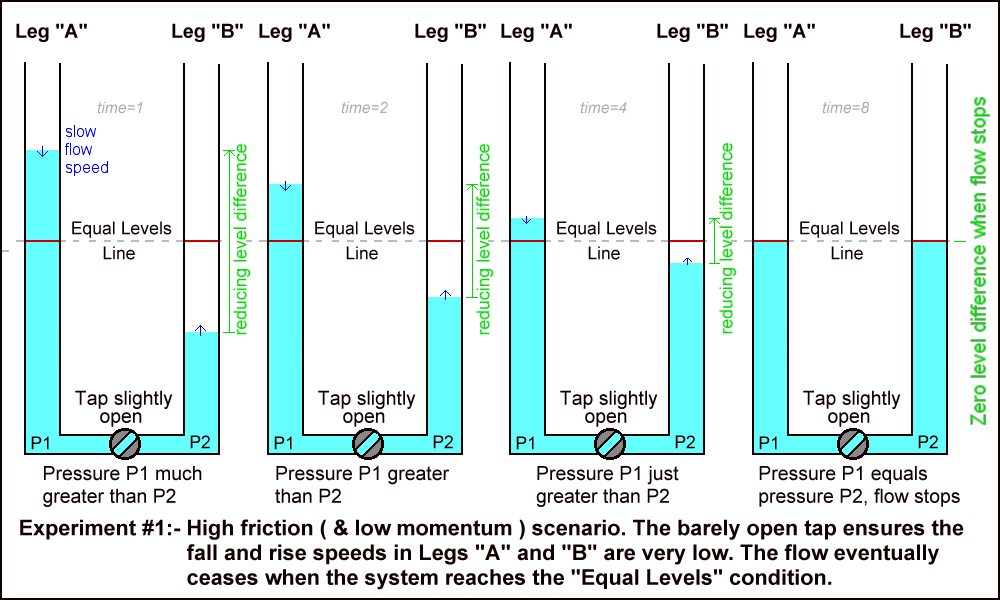
Frictional drag occurs whenever water flows over a solid surface. However it is largely confined to the water layers closest to the solid surface, and of course grows proportionately with the amount of surface area involved. In this experiment the U-tube tap is only opened by the smallest possible amount to give just a slow leak.
While the surface area of that restriction remains small, all of the flowing water is forced to flow through this narrow high friction region so all of the water experiences the high level frictional drag force. It is therefore classified as a high friction flow.
However because the rate of flow is very small, it will take a long time for the flow to finish. The very low flow rate ensures that the water speeds in either leg are always very small and so the momentum developed by the moving water will be limited to insignificantly low levels. This diagram outlines the evolution of system until the flow stops:-
In this experiment, after a new "set-up" sequence, the tap is fully opened at time=0. The flow through the wide open tap suffers much lower frictional losses because much of the flow passes through the middle of the tap opening and away from its walls.
The water then begins to drop in Leg "A" and rise in Leg "B". Due to the inertia of the mass of water involved, this movement begins slowly but accelerates to a more rapid pace. This diagram outlines the evolution of this second experiment using a fully opened tap:-
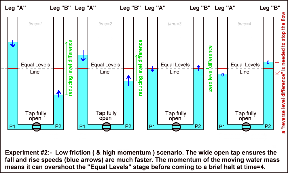
At time=1 the dark blue arrows indicate the size of the velocity achieved in each leg. The flow is much faster than in experiment #1 because the flow friction experienced through the wide open tap is much less.
At time=2 the water velocity has increased further, even though the level difference ( green arrow ) has decreased considerably since time=0 and time=1. This is because at the beginning of the flow a lot of the level difference force is used up in just getting the water moving from a "standing start". Over this period a small part of the original gravitational potential energy has been dissipated by the low friction level, but a much larger part has been converted into the growing kinetic energy of the accelerating water mass. The flow may actually reach its maximum velocity around this time.
At time=3 the levels in both arms have reached the "Equal Levels" Line but the water is still moving down Leg "A", through the cross tube and up Leg "B" because it has retained some of the forward momentum acquired during the earlier stages of this experiment. Many may ask how is it that the flow still continues, with water pressure P1 higher than P2, even though the height of the water in each leg is the same?
The answer here is that although at time=3 the water pressure at the bottom of each leg created by the downward gravitational forces is the same in each leg, there are additional dynamic forces involved that add to the bottom pressure in Leg "A" and subtract from the bottom pressure in Leg "B". A dynamic force "F" is involved anytime a body of mass "m" changes its velocity at a rate "a" (a= acceleration rate). Sir Isaac Newton discovered the relationship between them is: ( F = m times a ) and this is one of the fundamental Laws of Motion.
If a body is to increase its velocity (ie. accelerate), its surroundings must supply the extra dynamic force to achieve this. Conversely if a body decreases its velocity (ie. decelerates), then the body exerts the extra dynamic force on its surroundings as its momentum (= mass times velocity) is being reduced. The direction of these extra forces is in the direction of motion.
Now the water in Leg "A" is reducing its downward velocity as shown by the shortening blue velocity arrows after time=2. This creates an extra downward dynamic force at the bottom of Leg "A" in addition to the downward gravitational force, and so raises the water pressure P1 above that due to gravity alone. At the same time the water in Leg "B" is reducing its upward velocity as shown by the shortening upward blue arrows. This creates an upward dynamic force in Leg "B" that counteracts a part of the downward gravitational force there. This decreases water pressure P2 below that due to gravity alone. Since the water pressure P1 remains above P2, even though the heights are the same, the flow from Leg "A" into Leg "B" still continues at the "Equal Levels" time.
You may note similar "dynamic force" effects in tall buildings with high speed lifts. When the lift is moving downwards and begins to decelerate approaching your destination floor below, you will feel above normal forces in your legs and ankles as your body is being slowed to a halt. When the lift is moving upwards and begins to decelerate approaching a destination floor above, you will feel lower than normal forces in your legs, ankles, and possibly stomach, as your upward body velocity is being slowed to a stop. If you were to stand on a set of bathroom scales inside that lift, you would easily see a significant change in your "apparent body weight" in these two different situations.
The left-to-right flow through the horizontal connection continues beyond time=3 creating a growing "reverse level difference", now in the opposite direction. This is shown by the red arrow which grows from time=3 until all the forward momentum of the flow is completely dissipated and the flow ceases at time=4.
This is the time of "slack water" in the U-tube system, where the reverse height difference between Leg "A" and Leg "B" has grown sufficiently large so that its reverse force level just counteracts the forward dynamic force generated by the decelerating water mass. This leaves P2 and P1 momentarily equal with no flow through the connecting channel.
At this no flow, no momentum point, the dynamic forces then disappear leaving P2 higher than P1 due to the extra water height in Leg "B". Under these conditions the water flow begins to accelerate in the reverse direction, with the excess of P2 over P1 supplying the dynamic force that the now reversed and accelerating water mass requires.
The system may undergo a few smaller oscillation cycles before settling down to the "Equal Levels" condition. Note that if it were possible to entirely eliminate friction, the U-tube oscillations would be large and be never ending. It is the presence of the frictional drag forces that dampen the system and determine the level of the first overshoot (if any). It is the ratio of the system's momentum levels to the level of friction that determines the time delay of the first "Slack Water" moment with respect to the time of the first "Equal Levels" moment.
The gravitational, frictional, and dynamic forces described in the U-tube experiments are generally applicable to any two tidal water bodies connected together by some form of a channel. Note that although the origin of tides in the ocean is connected to the position of the Moon and Sun in the sky, these relatively weak tide raising forces are only effective over large ocean scale water bodies. So for bays and harbours it is only the "outside" level that is "wobbled up and down" by celestial body forces. Tides that arise on the "inside" waters are just manifestations of how the water currents through the entrance accelerate and decelerate back and forth in response to the "outside" tide level changes.
We saw in Experiment #1 (high friction and low momentum scenario) that the "slack water" moment of no flow arrives at the same time as the "Equal Levels" moment. In Experiment #2 (low friction and high momentum scenario) the water flow was seen to "overshoot" the "Equal Levels" point by quite some margin, creating both a time delay before slack water occurs and a growing reverse level difference before the flow actually halts.
Sadly, almost all commentators on Port Phillip's tides and entrance currents simply assume it exhibits Experiment #1 type behaviour without actually checking if this is true. They then go on to totally ignore the mass of water involved and assume no dynamic forces are in play. They therefore describe the behaviour as entirely determined by the flow friction levels for each particular value of the "outside" to "inside" level difference force. This is the "simple story" put out by nearly all government departments and is copied widely by boating related organisations around Port Phillip.
Despite many requests, it has been impossible to determine whether the port authorities actually believe in what they are saying is true, or whether are just putting this out as, what in their view is, a "harmless simplification". The posts on this website are mainly aimed at getting a more accurate understanding of the tides and streams near Port Phillip Heads, and also pointing out that this common "simplification" is not in fact "harmless". It fosters untrue and unsafe ideas about the current versus time profile at Port Phillip Heads, and so raises risk levels.
As the size of bays or estuaries become larger there is a tendency for the mass of the water involved in tidal streams to grow more quickly than the friction levels that oppose those flows. This is because the first grows in proportion to the channel volume while the second grows in proportion to the surface area of the channel seafloor. The bigger a waterway is, the more prominent its inertia and momentum effects will be.
Port Phillip stands out from most other bays and harbours in that on average a whopping billion tonnes of sea water flows in or out every six or so hours. The speed of these massive flows can also be up to 10 kph. These properties alone put Port Phillip well into the Experiment #2 camp where, at least at the lower water speeds, the dynamic forces required to accelerate and later decelerate the large water mass become dominant over the system's frictional drag forces. The dynamic forces involved totally alter the way the level difference driving forces get translated into tidal stream speeds compared to the common "simple view" where the dynamics is totally ignored.
Numerous in-the-field observations of Port Phillip show that by the time the "Equal Levels" moment occurs, the weakening tidal current through the Heads is still running forward at between 1 and 2 knots. The residual forward momentum still in this billion tonnes of slowly flowing water is sufficient to propel the water forward for a further time period between 35 to 95 minutes depending on the exact sizes and sequence of the tidal cycles.
The evidence also shows that the strongest of tidal streams produce a reverse level difference of around 30 to 40 cm before the flow briefly stops to produce slack water. The maximum reverse level difference at this time is then quite significant at around 30% of the maximum forward level difference that drove the fast 6 knot tidal currents some three hours earlier.
The high reverse level difference existing at slack water time also helps the new reversed tidal stream accelerate away far more quickly than for the incorrect "equal levels and slack occur together" style of thinking that is very wide spread and hard to dislodge. It is that incorrect understanding of the proper current vs time profile, particularly near slack water time, that is the main danger of the common "simple view" of Port Phillip Heads.
All our understanding of the mathematics of seawater flows around coasts and bays can be incorporated into a computer model of the waterway to be studied. Such models divide the waterway into a large number of cells, with each cell representing one small part of the waterway. Each of the many cells is also given a water depth, bottom friction characteristics, and several other parameters that may later help to "tune" the model by checking its final output against measurable parameters at various points in the real waterway. Constructing the model is a task where compromises must be made. Using more cells to improve the spacial resolution of the model results in longer computation times and the need to have more accurate waterway bathymetry.
The computation phase starts with using known tidal information, gained by other means, applied to the cells along the open ocean boundary of the model. This open boundary is usually well outside the area of interest and in areas where the tides are simpler and well established. The effect on the next inner adjoining layer of cells is then computed using a set of equations that describe the flow through those cells, taking into account the dynamic forces and several fundamental conservation laws of fluid mechanics.
The computations then move to the next adjacent layer of cells and so on until all cells have been covered. To allow for all interactions between model cells, the process is repeated with exactly the same open boundary input values until all cells yield stable values for water flow in or out of each cell. This completes just one model "time-step". Values of interest can then be extracted from the model and stored for later use. New boundary conditions to suit the next time-step are then input, and the whole computation process is performed again on these new inputs. The behaviour of the whole waterway in response to the time varying boundary conditions gradually emerges from the model. The extracted data values at each time-step help in understanding the "inner workings" of the real waterway.
Of course the faithfulness of the model's results to "the real thing" is affected by the compromises made along the way to reduce the often long computational running times. These compromises may include the cell size and the time-step intervals. Early PPB models may have used cell dimensions of a few km and time-steps of one hour. Time steps of this size are adequate for a general overview description of the build up and decay of tidal currents through the Heads, but can miss catching the details of the growth of the reverse level period leading up to slack water as this phase can be less than one hour long.
I have used data from a low resolution hydrodynamic model of Port Phillip to create an animation to help visualise both the sea level and tidal current behaviour. The model's cell size is just a little too large to give completely faithful current values, but the time-step interval of 30 minutes was smaller than for many other models. To make for a smoother animation I have created two extra 10 minute "data points" using linear interpolation between the 30 minute data points. This is justified on the basis that most of the parameters discussed in these posts do vary close to linearly with time around the period of most interest which is near the slack water time.
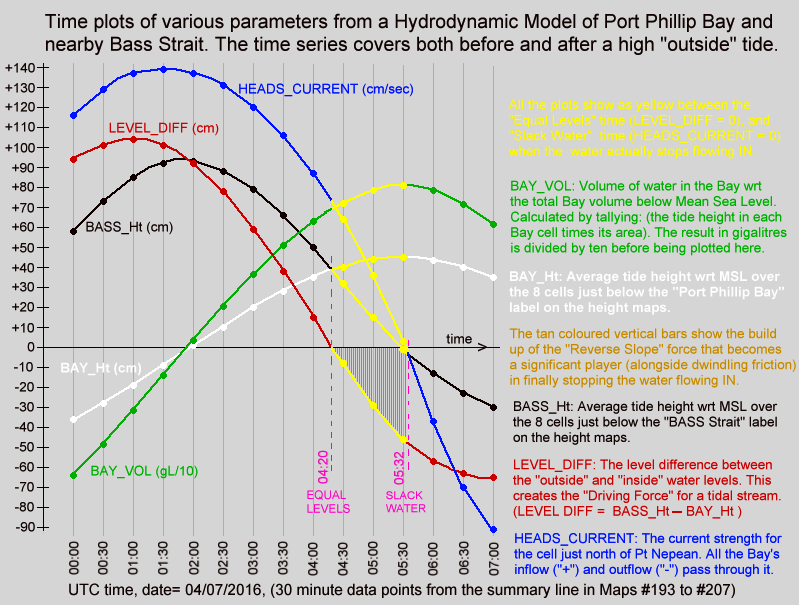
Hopefully this reasonably truthful graphic presentation may help in understanding the large inertia and momentum effects on the current's behaviour that are ignored in the "official advice". The relationship of both the sea level differences and the currents to the "Equal Levels" and "Slack Water" moments are the most important offerings of this model:-
Twin "maps" of Port Phillip are shown, with colour coded sea level heights on the left map and colour coded current speeds and direction on the right map. The lower section shows graphical plots of the "outside" (white) and "inside" (red) sea level heights. Each height is taken as the average value of a cluster of cells around the white and red locations mark with a *. The lowest plot is of the level difference (Bass_Ht - Bay_Ht) that provides the driving force for the tidal currents. This shows as green during the long down-slope current flow, and as red for the shorter up-slope phase.
It is this level difference that drives the Bay's currents and tides. When one side is higher than the other, water pressure differences create a horizontal force that acts on the enormous water mass between the ocean and mid-bay regions. However this force, modified by the frictional drag and dynamic forces, only determines the rate of change in the water's speed and does not in itself directly determine the resulting speed, or indeed the direction of the water flow. ( Acelebration = Force / mass )
The level difference is a measure of the strength of the applied "driving" force. Forget the Moon & Sun, they serve only to wobble the "outside" ocean level up and down, and have no direct gravitational effect on water bodies the size of Port Phillip. Tidal streams at the entrance, and tides within Port Phillip Bay, are all the result of these level difference forces pushing a large mass of water back and forth while also overcoming various frictional resistances. These inflows and outflows alter the volume of water residing in the Bay and hence make its internal tide heights rise and fall.
The animation's blue plot shows the resulting current velocity through the Heads. Positive values indicate a flooding (inward) current. Note that the slope of this blue curve is at its steepest as it passes through the slack water times. This is in complete accord with actual current measurements, but is in fact the exact opposite of the assumption that logically follows from the official "simplified advice", where it is claimed there is no level difference at slack water, and so no forces that can change the current's speed quickly. In particular note the change in current speed around slack water is approximately linear over time, and does not have a low-speed "flat-ish profile" at slack water as many folk assume.
The yellow plot shows the variation over time of the volume of water residing within the Bay relative to its volume at Mean Sea Level (MSL). Naturally it's minimums and maximums correspond to the slack water times. The changing numerical values of each plot point are shown as coloured numbers below the maps.
This fairly low spacial resolution model exaggerates the up-slope phase slightly because its in and out mass flows calculate out as a little larger than in the real life Bay. This is due to the entrance being modelled by a slightly too wide single cell. In the real Bay, the up-slope flow times are more typically observed to be in the 35 to 80 minute range. All the main features of the Bay's water flow are reasonably represented here, but the data shown is just a small subset extracted from a much larger scale "all of Bass Strait" hydrodynamic model produced by the Tasmanian tidal modelling company "TideTech". The much newer CSIRO national tidal model does have better spacial resolution, but its complex unstructured pattern of cells puts animation of its data way beyond my programming skills.
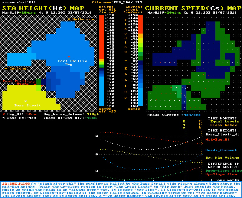
The animation shown above had its colour banding for sea height set at 15 cm per band so the whole cycle could be accommodated in the limited colour pallette available. The two static images below are of "slack after flood" and "slack after ebb" respectively, but with a finer colour banding set at just 5 cm per band. These better demonstrate the physical extent of the reverse slope regions at slack water time.
"Slack after FLOOD"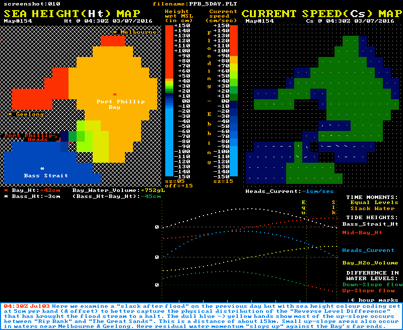
Note also that the graph section of both images shows that at the "Equal Levels" moment (yellow time line), the Heads current is still flowing with some strength. It is the residual momentum in the tidal stream at this time that powers the up-slope flow phase until slack water is reached (orange time line). Again note the speed of the current changes most rapidly around the slack water times.

There is also a static image of a sequence of eleven commented screenshots at this link: See 11 frame sequence.
This may render as a tall and skinny image, in which case the image will need to be "clicked" to bring it up to full width. The commented frames can then be scrolled through one at a time at your own pace, giving you time to read the commentary while referring back to either the maps or graphs to fully understand the blue text in the comment box.
Yes there are a few I know of and perhaps even more I don't know of. The physics of stopping and reversing a tidal flow is the same everywhere. To slow it down and then bring a tidal stream to a halt requires a force in the opposite direction to the flow. While frictional drag is a big player in this task at the higher flow speeds, for every halving of flow speed this achieves, the drag force diminishes to just a quarter of its previous value. Fictional drag is never going to bring the stream to a halt (in a reasonable time) by itself.
All streams will therefore overshoot the "Equal Levels" point to some extent and so rely on a Reverse Level Difference force to bring the tidal stream to a halt. The question is then whether the associated up-slope flow time is long enough to be noticed in any practical sense for boating folk.
While many locations in Australia can experience fast tidal streams at the entrance to bays or estuaries, or in other channels connecting water bodies, that in itself is not sufficient to see lengthy up-slope tidal flows. There seems to be three necessary geographic ingredients for this to occur. I estimate these at roughly:-
1) Fast(-ish) peak tidal flows (say > 3knots).The frictional drag characteristics of the constricting channel, combined with points 1) & 2) determines how much residual forward water momentum remains at the "Equal Levels" time. Narrow channels with their relatively high drag character generally mean "not much residual forward momentum", while wide and fast flowing channels mean "plenty of it".
Whatever that level may be, the duration of the up-slope flow time until the flow stops is then determined by the rate at which that momentum is dissipated. In turn this depends of the rate at which the reverse gradient of the up-slope phase grows. This leads to the rather anti-intuitive result that the faster tidal streams, which are produced by large range tides, have shorter up-slope flow times than weaker tides do. This is because those rapidly changing "outside" levels also mean a rapidly growing Reverse Level Difference which effectively "applies the brakes harder".
While it might be thought that faster streams should have much higher residual forward momentum levels, this isn't really that significant because of the much higher friction levels at higher speeds. These dissipate a lot of the forward momentum of fast streams before we even get to the "Equal Levels" point. Another "levelling" feature is that in the weaker streams, the "Equal Levels" time comes much sooner after the maximum speed point than it does for stronger streams. This means the weaker streams lose less forward momentum over that particular time interval than the stronger streams do.
The final ingredient "3)" as to whether a particular location experiences long up-slope flow times is the physical length of the "choke zone" constriction along the flow direction. The real "stopping power" during the up-slope flow period is the absolute slope in the sea surface. This is the Reverse Level Difference per kilometre and not the total level difference over the "choke zone". This means a long "choke zone" length will require the level difference to grow for a much longer time to achieve the required absolute surface slope to halt the flow. Conversely for bay/estuary/harbour entrances or other constrictions where the "choke zone" is quite short, sufficient surface slope to finally halt the flow might only take a handful of minutes to develop. In that case the "Equal Levels" time and the "Slack Water" time are not discernibly different.
While there must be hundreds of Australian locations satisfying condition "1)", it is conditions "2)" and "3)" that severely narrow the field, taking out places like Solway Pass (QLD), and Hells Gate (TAS). Closer to Port Phillip is the neighbouring location of Western Port (Westernport Bay). The first sea level and current map set below is taken from CSIRO's tidal model and shows the situation at the Equal Levels time in Western Port:-
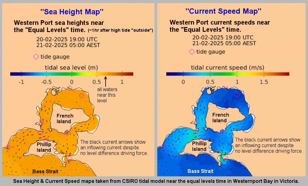
The second map set shows the situation near Slack Water time:-
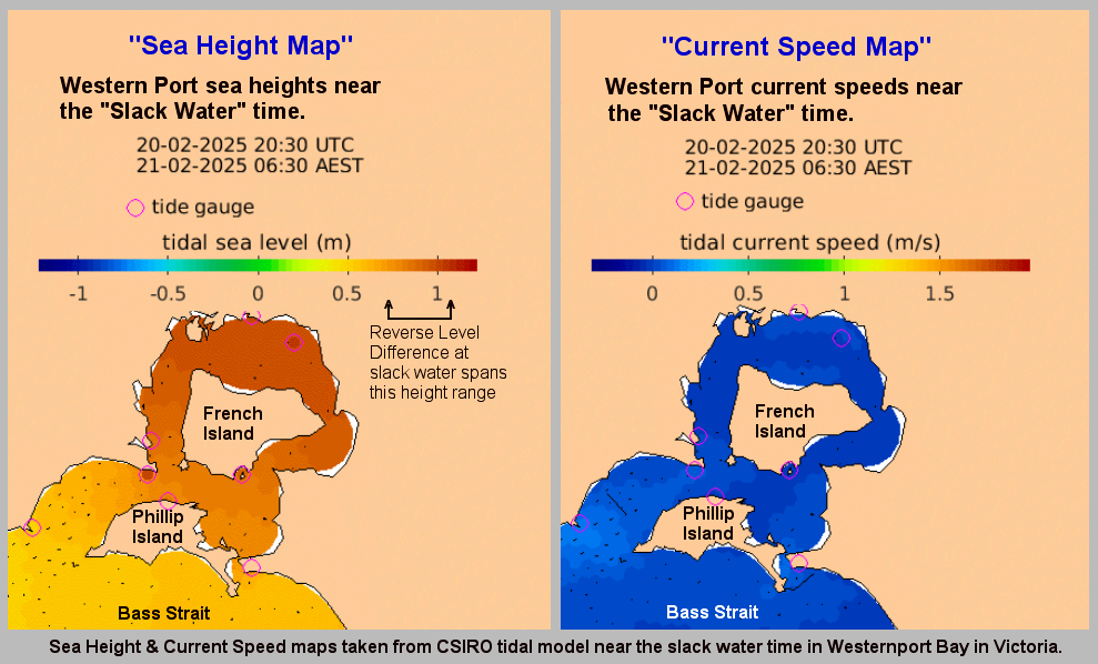
The CSIRO modelling also shows up-slope flow in a number of locations in Bass Strait between various islands and the mainland. There are also hints of it in Backstairs Passage that separates Kangaroo Island from mainland South Australia. However the most significant tidal momentum effect of all seem to occur in "Banks Strait" off the northeastern tip of Tasmania. Here strong tidal flows run through a 20 km wide gap between the northeast tip of Tasmania and the southernmost islands of the Furneaux group. A location map for Banks Strait is shown below.
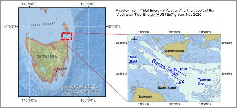
This area has been extensively studied as a potential site for "tide turbines" for electricity generation, and so the modelling is well verified. Although the maximum current speeds through this strait are somewhat lower than through Port Phillip Heads, the width and depth of the strait means the momentum levels of its tidal streams are much higher than Port Phillip's, while the relative friction levels are lower. In this high momentum, low friction waterway, the time delay between the "Equal Levels" and "Slack Water" moments is typically around 2 hours. The Reverse Level Difference at slack water is typically around 70 cm. An animation loop of some of the modelled sea level and current speed data is shown here:-
Of note in this waterway is that the tidal current speed at the "Equal Levels" time is still around 70% of the maximum speed reached earlier in the cycle. Also of note is that the shape of the blue current plot again shows the most rapid changes in the speed of the tidal current occurs around slack water time.
There is a larger scale static graph at this link:- Banks-Strait-Plots
This webpage has shown that "simple stories" which try to describe tidal flows only in terms of water level differences significantly miss the mark for waterways where large mass flows occur. To ignore the dynamic forces needed to alter the speed of the water mass gives a inaccurate and potentially unsafe description of the tidal behaviour. In any tidal waterway the current flow will not be stopped by the time the "Equal Levels" point is reached (as is often claimed), but can continue forward for some further time, driven onwards (and up-slope) by "cannibalising" its own residual forward momentum.
The duration of that up-slope flow until slack water is reached depends heavily on the size and shape of the waterway, and also on the details of the varying tidal patterns that drive the flow. Variations in the tidal patterns only repeat closely every 18.6 years, so at times it can seem like there is "endless" variability between one slack and another. A useful discussion of this variability in Port Phillip's tidal streams is given in POST #0_C. You can either start at right at the top, or possibly skip forward to the heading:- "Tidal Stream Overview". The histogram plots in particular are a simple tool for understanding the range of things Port Phillip Heads may serve up at different slack water occurrences.
At the bottom of POST #1 there is a link to the CSIRO tidal model results, and some basic instructions on how to use it to examine various selected tidal areas. Further up in POST #1 is a heading Stopping Flowing Water - the "Water Hammer" Effect. This is really a discussion of tidal dynamics in "plumbers terms". These water hammer principles can be quite useful for quickly understanding the situation during the deceleration phase of a Port Phillip tidal stream where folk are often confused by finding an inflowing current at the Heads but with a falling tide, or an outflowing current but with a rising tide.
If you arrived here by following a link from the Index Page, just close this page to return to the Index to see the other links to related posts.
If you arrived here via an external link, you can visit the site's Index Page with this link: Jake's Index Page
--------------------------------- The End ----------------------------------