This POST #3 looks in more detail at the small slopes in the surface of the sea that drive the tidal currents in Port Phillip.
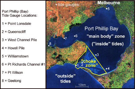
The flow of sea water in and out of Port Phillip is partially choked by both the narrow entrance and the large shallow areas between 5 km and 15 km inside the entrance. Beyond this "choke zone" the Bay's main body (or "inside") tides have a range of only 30% to 60% of the "outside" tidal range.
The lower percentage figure applies to the fastest flowing tidal streams which suffer proportionally more "choking" than the gentler tidal streams do. The High and Low times of the "inside" tides also occur around 3 hours after the "outside" times. Both these factors create a time varying difference between the "inside" and "outside" water levels, and consequently a time varying sea surface slope across the "choke zone" which stretches over about 15 km from "Rip Bank" just outside the Heads, to the northern edge of the "Great Sands" area.
The weight of the extra water on the high side of a sea surface slope produces slightly higher water pressures at all points under that location compared to the horizontally corresponding points under a location further down the slope. This small sideways water pressure differential, acting down through the entire water column, produces a net horizontal force that acts on the water under the sloping surface. The strength of this horizontal "slope force" rises in direct proportion to the size of the surface slope but it always acts in the directly down-slope direction.
The way the water responds to this slope force depends not only on the drag generated by bottom friction and turbulence while the water is moving, but also on the water inertia or water momentum effects while the flow is gaining speed or losing speed. These latter effects are quite significant in Port Phillip because of the very large mass of sea water involved in its tidal movements compared to most other waterways. On average, around a billion tonnes of water gets firstly accelerated and then decelerated as the tidal current through the entrance firstly speeds up and then slows down during the approximately 6 hour run of each tidal stream.
Sadly, many or most commentaries on Port Phillip's tidal currents ignore this important water mass aspect, where a sizeable part of the slope force is related only to changing the water's speed rather than overcoming frictional drag. Instead they promote an incorrect view that the current's speed is almost entirely related to frictional factors, and so is directly related to the level difference or slope force. This gives readers a very much poorer understanding of this system, particularly during the approach to slack water where the current slows, stops, and then reverses. Unfortunately the wide promotion of misleading information about this important period raises the level of risk for recreational boaters operating anywhere within the "choke zone" region of Port Phillip.
The slope forces, modified by friction and inertia or momentum effects, are what drives the tidal currents both at the Heads and further inside Port Phillip. The role of the Moon and Sun is essentially restricted to just wobbling the "outside" level up and down. It is the slight difference between the current strength "on the Heads side", and "on the Melbourne side" of any particular location that determines whether the amount of water around that location is increasing or decreasing. In turn this dictates whether that location's tide height is rising or falling at that particular moment in the cycle. This gives a progressive delay of up to three hours in the Hi/Lo tide times as we move inwards from the Heads and into the main body of the Bay.
The level difference across the "choke zone" may reach up to 120 cm when the tide is flowing strongly. This gives an average downward sea surface slope of around 8 cm/km, but slopes nearer the Heads may be up to as much as 15 cm/km, with lower than average slopes closer to the main body region where the flow speed is much lower. Even the highest slopes are not visible to the naked eye but are more than sufficient to produce fast downhill flows either in or out of the Bay.
Note that boaters who pass close to the edge of the drying reefs of either headland while the water is flowing fast will often claim they can "see" a 40 to 50 cm water level difference over just a short distance. However these observations are not the tidal stream driving slopes, but only a localised "bow wave" effect. From the flowing water's point of view, the reef rocks are "speeding though it at 4 to 5 knots", and so create a bow wave of similar height to a boat moving at that speed through stationary water. The real slopes that drive the tidal streams through the entrance remain invisible to the eye but are easily observed via the Bay's tide gauge network.
Most boaters are very comfortable with the concept of a water current "running down a water slope" through the Heads. However, they are far less comfortable with the concept of the current "running up a water slope". The latter does occur as a "water momentum effect" in the final phase of a tidal stream's flow. The duration of the up-slope flow varies typically between 35 to 80 minutes, depending on the tide sequences.
During this time we have a growing reverse slope force so that at slack water the reverse level difference across the "choke zone" may have reached 40 cm or so. This fairly high level of slope force brings the tidal stream to a halt rather abruptly. This is important, because not understanding this effect leads many recreational boaters to assume the wrong current versus time profile around the time the current reverses. The commonly assumed "mythical current profile" is far more benign than the actual one, so these folk are put at higher risk.
Unfortunately over many decades the port authorities, along with many other organisations and individuals, have incorrectly claimed that the tidal current reverses direction as soon as the surface slope reverses. (ie. they claim no slope force exists at slack water time). While it may have been thought this claim is a "harmless simplification" of the real situation, it reduces many boater's understanding of the Bay's tidal streams, and unwittingly exposes them to increased risk in this region (see POST #1 on this website).
Although this "simplification" is very widely accepted and believed, it makes no more sense than claiming a skateboarder rolling down the slope on one side of a skate bowl will stop at the bottom of the bowl (driving force = 0), and is therefore unable to keep moving forward to roll up the slope on the opposite wall. Any mass with some forward momentum, be it a skateboarder, or a child on a swing, or a cricket/golf/tennis ball, or a billion tonnes of moving sea water, can climb upwards against the force of gravity by sacrificing some of its speed and momentum in order to do so.
Another method of better understanding the behaviour of Port Phillip's tidal streams is to construct a time series of the sea surface heights that exist along a transect line that starts outside the Heads, runs through into the main body of the Bay, and then on up to Melbourne. This would show the development over time of the "down-slope" and "up-slope" phases of the current flow during each tide cycle. It would also reveal the strength and direction of the gravity related forces that either assist or retard the flow of the tidal stream.
Ideally this could be done by hydrodynamic modelling which could yield closely spaced points along the transect. As far as I am aware no modelling group has done this for Port Phillip over a full tidal cycle. Instead I have attempted a poor man's manual version of this by using a five point transect line through parts of the Bay's tide gauge network.
This "not quite straight" transect line is shown as the green line in this image.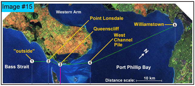
Note this map has been rotated 45 degrees clockwise from the usual "north-up" orientation. This allows the transect to be approximately horizontal across the important "choke zone" (2 --> 4). The pink lines are verticals dropped down from the five monitoring points. The time series of tide heights will later be plotted progressively down these lines and then joined across to give a series of "snapshots" of the sea surface slopes along the transect as they change over time.
The "outside tide" at around 5 km outside the Heads is taken as the Lorne tide height but delayed by 6 minutes. Data for the other four points of the transect are from selected tide gauge locations from Pt Lonsdale through to Williamstown. Those raw gauge height numbers are first corrected to the Australian Height Datum (AHD) before the points are plotted. This ensures the slopes drawn between plot points then represent true sea surface slopes.
Although the predicted or observed tide heights (wrt AHD) at various times are sufficient to construct a series of plots showing the surface slopes, their value is much enhanced if the corresponding inflow or outflow rate through the Heads is also available. To this end I have used my water volume modelling work that subdivides the surface area of the Bay into a number of zones, then estimates the changes in water volume by multiplying the area of each zone by the appropriate tide height for that zone at each 6 minute time point. Note these calculations deliver the net change in water volume relative to the total water volume Port Phillip would have at a uniform water level equal to the Australian Height Datum.
The most sensible units to use for these volume changes are gigalitres (= 1 million cubic metres) because of the simple relationship that a tide rise of 1 metre requires exactly 1 gigalitre (gL) of extra water for each square kilometre of water surface. Therefore in rough terms we might expect that with a maximum tidal range of say 0.9 m, over Port Phillip's area of around 1930 km2, the corresponding change in water volume will be in the order of 1,560 gL. Small tide cycles may have water volume changes down to around 400 gL.
The difference between the volume numbers at the successive 6 minute calculation points can be converted from a volume change rate into an average current passing through the underwater cross-section at the entrance. This is done by dividing the volume flow rate by an estimate of that cross-section. This is an area of complex bathymetry, but a guesstimate of around 36,500 square metres was obtained.
This gives entrance current values averaged over the entire entrance cross-section, and so are lower than the official "peak stream rate" predictions published by the BoM & AHO. Those are for the shipping channel centre line, which avoids much of the bottom friction effects of the shallower reefs in other parts of the Head's cross-section. To "boost" my calculated current values to numbers closer to the official predictions, a reduced effective cross-sectional area of 30,000 square metres has been used in this work. In practice the slack water times delivered by this water volume modelling approach usually fall within 10 minutes of the official predictions.
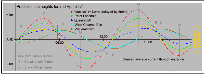
In Image #16a, the top panel shows a time plot of the predicted tide heights (wrt AHD) for the five transect points. It clearly shows four times where the tide curves all intersect at the "Equal Levels" times, where the sea height across the entire Bay and out into the ocean is briefly all at the same level. These times are also "zero slope" and therefore "zero driving force" times.
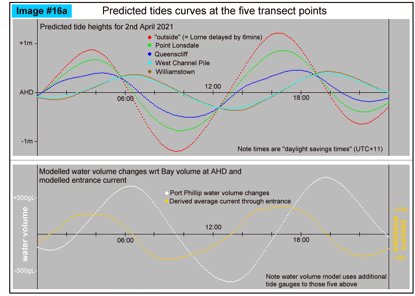
The lower panel shows the modelled changes in the water volume curve (white), plus the entrance current curve (yellow) derived from the gradient of the water volume curve. It is clear that "Slack Water" (zero current) occurs quite some time after each "Equal Levels" time. This is in accord with POST #1 which outlines the effects of momentum levels in Port Phillip's high mass tidal streams. The simplified and false "official line" which claims that "Equal Levels" and "Slack Water" occur at the same time is out of step with reality and hopefully will be amended one day. (It is also out of step with the official slack water time predictions produced by the BoM which are used successfully by thousands of recreational boating folk each year).
The date of 2nd April 2021 was chosen because any weather effects on the real tides tend to be less in the more stable Autumn months. In addition this particular date features large tidal ranges and also has the advantage of the first "equal levels" time being in the first few minutes of that day. The small jitter in the entrance current curve in the bottom panel is caused by the 1 mm quantisation of the tide height predictions. The inherent rounding up or down to the nearest millimetre produces small "bumps" in the volume curve. In turn these translate into some jitter in entrance current values that are derived from the slope of the water volume curve.
Image #16b below shows the results when the modelling uses the observed real tide heights rather than the predicted heights. The observed tide curves are in general similar to the predicted curves with some minor "weather wobbles" related to changes in the "tidal surge" levels that are caused by air pressure changes and various wind and wave set-up conditions in Bass Strait. Varying surge levels of up to +/- 15 cm are common even in mild weather conditions. Much stronger (storm) surges from +40 cm to +80 cm also occur perhaps a dozen times per year in the most boisterous weather conditions.
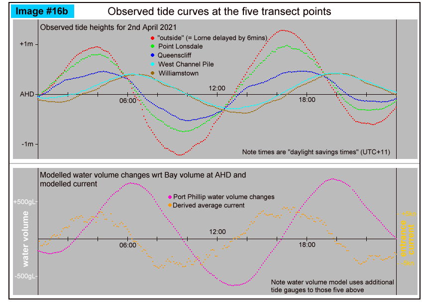
The lower panel shows the modelled volume curve (pink), and the entrance current derived from it as the orange plot points. The large current jitter highlights the weakness of this method for entrance current determination from observed tide curves. Local weather effects at a gauge site lead to a lack of smoothness in the volume curve, which gives rise to large jitter in the entrance current plot. Most of this can be tied back to the "weather wobbles" apparent in the Williamstown tide curve in the upper panel. Since this curve is used in several large area modelling zones, the overall effect on the derived entrance current values can be severe.
Nevertheless both sets of plots agree in their general features and both show that the maximum and minimum water volume times (ie. the slack water times at the Heads) occur quite some time after the "equal levels" times. Again this fully supports the main arguments of POST #1 on this website that:-
i) tidal streams halt well after the "equal levels" moment.
ii) a significant reverse level difference between the "outside" and "inside" waters develops by the time slack water occurs.
iii) the speed of the entrance current changes almost linearly with time around slack water, and that rate of change is higher than at any other time in the tidal cycle.
Grasping the last point is important in re-educating recreational folk away from ideas they may have inferred from the incorrect "official line" statements that at slack water there is no surface slope and hence no forces in play. This misinformation appears to encourage many recreational boaters to go on to assume that the entrance current won't be changing quickly around slack water. That erroneous assumption puts them at higher risk when operating in this potentially very dangerous area.
Also of note is that although the tide curves themselves, and the (not shown) "drive level" curve are approximately sinusoidal in shape, the entrance current curve is far more flattened near its extremes. This is in part due to the maximum current speed rising as the square root of the drive force because the frictional drag rises quickly as the current's speed grows.
The results using the predicted tide curves for the entrance current modelling shows that at the four "equal levels" times, the tidal streams are still flowing at between 1.5 and 2.2 knots. The "up-slope flow times" until slack water are given by the modelling as: 54, 42, 48, and 36 minutes respectively. The reverse level differences at slack water are: 29, 40, 39, and 31 cm respectively.
Compared to the slack water predictions from the BoM (by Cardno) the modelled slack water times here are a little earlier by: 12, 3, 13, and 8 minutes respectively. The later Cardno slack water times imply longer up-slope flow times of: 63, 45, 62, and 43 minutes respectively. The reverse level differences at the Cardno slack water times would also be larger at: 35, 42, 52, and 37 cm respectively.
Image #17 below shows a "split screen" image showing dual copies of the Image #15 transect, to which height and entrance current data from the time plots of Image #16a (left side) and Image #16b (right side) have been added. It shows the average sea surface slopes along the 5 point transect for a series of selected times running down the screen. The timestamp and entrance current values are shown at the left end of each plot in yellow or orange.
The plots are at selected times of significant events as noted by black text in the left margin. Different height and distance scales are used to give a highly exaggerated view of the surface slopes. In reality these are just a small fraction of one degree.
The AHD level for each plot is shown by a dark grey line. The "inside" tide level wrt AHD is shown in yellow or orange text near the middle of each plot. That same level, but referenced to the "outside" level, is shown by the black text further to the right.
Due to the jitter problem with the current values obtained from the observed tide heights, the entrance currents for the "right side" plots are determined from a rolling 3-point average of the data points. This is then shown as a directed "current arrow" of the appropriate length, rather than as a number.
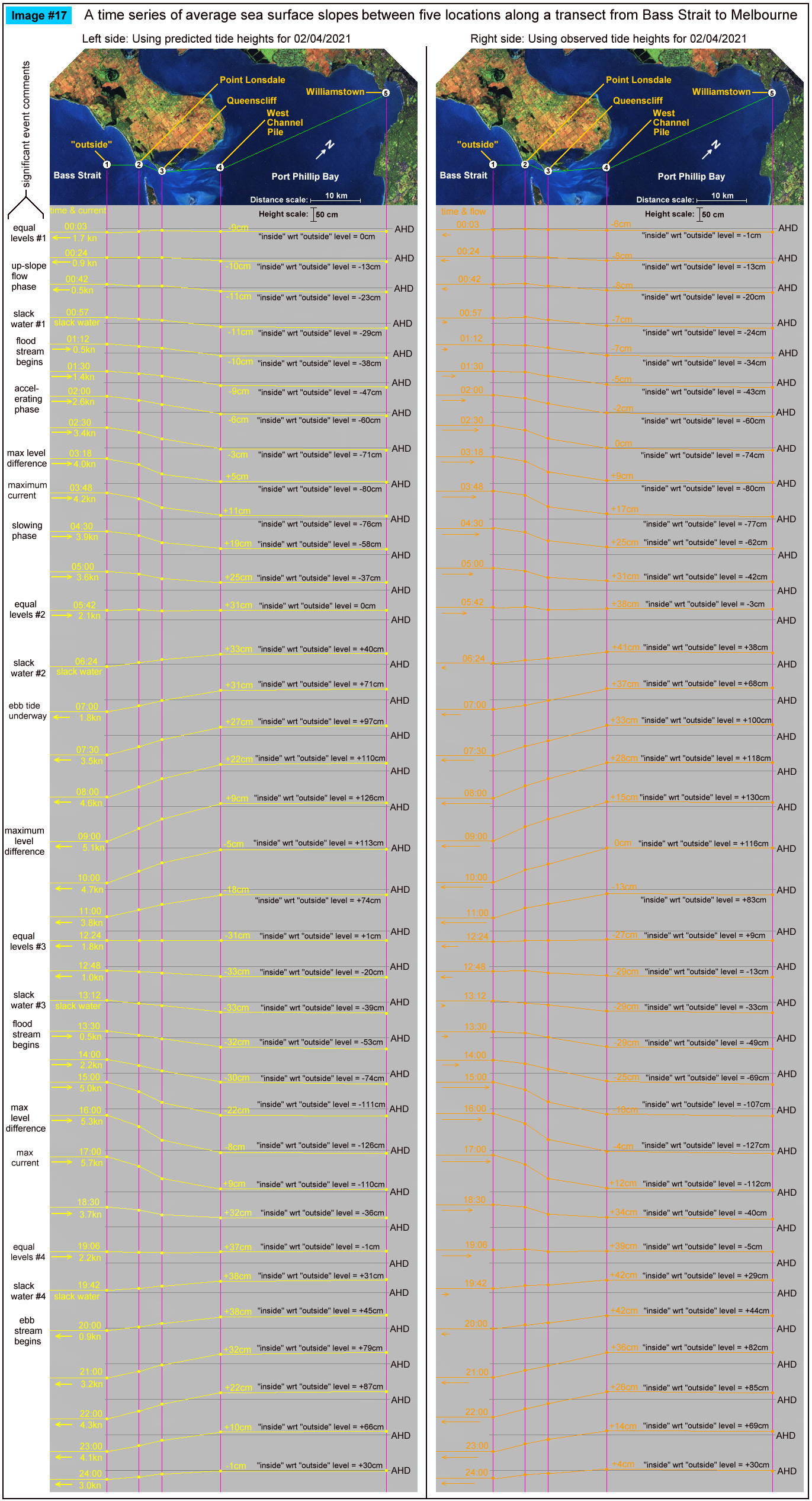
Points to note about the four "Equal Levels" and the four "Slack Water" times are:
a) The "Equal Levels" time is a rather extraordinary event with the sea surface at essentially the same level over some 75 km.
b) At that time, and with NO driving force in existence, the entrance current is still running at around 2 knots.
c) The residual forward momentum still in the tidal stream at the "Equal Levels" time can drive the current flow for a further 30 to 50 minutes.
d) The current only stops, and is ready to reverse, when the reverse level difference has grown to around 30 to 40 cm.
e) At 02:30am, a +3.4 knot current needs a level difference of 71 cm to drive it while the stream is accelerating. However later at 05:00am, where the
same stream is decelerating, a level difference of only 37 cm is needed to drive an even slightly higher current of +3.6 knot. Roughly speaking, the average
shows about 54 cm is needed to overcome the frictional drag component, while the dynamic force component is +17 cm during the acceleration phase,
and -17 cm during the deceleration phase. At somewhat lower speeds the dynamic force components begin to dominate the frictional drag component.
f) Across the "main body" of Port Phillip (eg. 4 --> 5), there are only very small surface slopes at any stage of the tide cycle as its level rises and falls.
In regard to the above "slope diagrams", the "outside level" height point was placed at a nominal 5 km outside the Heads. In retrospect, and after viewing the CSIRO's hydrodynamic modelling (link given near the end of POST #1), it is likely that "location 1" in the diagram above could have been placed at more like 2 km outside the Heads. This would significantly increase the surface slopes in that critical region from "Rip Bank" (just outside the Heads) to the Point Lonsdale gauge (just inside the Heads).
That being said, it is timely to remember that the slopes in the diagram above have been highly exaggerated to make them visible by using very different vertical and horizontal scales. In the real world these water slopes are just a dozen or so vertical centimetres over every thousand metres horizontally. This means their angles to the horizontal plane are only tiny fractions of one degree. However these tiny slopes are sufficient to drive very fast currents because the friction levels in a fluid are way way below those in any equivalent "dry land" situation.
A sea surface where waves and swell exist is characterised by jumbled mix of high angle up-slopes and down-slopes, producing a chaotically changing sequence of sizeable forces. However over periods of a few minutes, and distances of 50 metres or so, these forces will average out to zero, leaving only the horizontal force due to a persistent underlying small surface tilt to act on the water at and under that neighbourhood.
This horizontal driving force is used to perform several different tasks, mostly all at the same time. Firstly, part of that applied force is used to overcome the speed dependent frictional drag experienced by a flowing tidal stream. If the applied force exceeds the frictional drag, then some of the excess goes into accelerating the flow and increasing its speed and momentum (& frictional drag).
If the driving force later declines, the excess of frictional drag over the applied force will begin to decelerate the flow to a lower speed. In effect part of the frictional drag is then being overcome by the sacrifice of some water momentum (& speed), with the remaining part being overcome by the reducing driving force. In very high water momentum settings such as Port Phillip Heads or Banks Strait, a declining driving force may reach zero (equal levels time) before the speed of the tidal stream does. At Port Phillip Heads the residual tidal stream speed at the "Equal Levels" moment is typically in the range from 1 to 2 knots, and somewhat higher in the Banks Strait example given in POST #1.
From that point on, the driving force slope grows again but in the reverse direction. The sacrifice of speed and momentum is now used to overcome not only the declining frictional drag, but also the growing reverse slope force until the tidal stream's momentum is completely dissipated. This gives a brief zero speed moment before the stream reverses direction and accelerates away under the continued growth of the slope force.
A final component of the driving force is used to increase the kinetic energy of those parts of the water where the speed increases over distance rather than over time. This occurs where the tidal stream encounters some form of constriction in the channel it flows in. Where the channel widens this component is negative, and so assists the current flow rather than hindering it. This is thought to be the reason that when averaged over a large number of tidal cycles, the constricting ebb streams in Port Phillip run about 20 minutes longer and slower (in volume terms) than the expanding flood streams do.
Where all the components of the slope force are acting at the same time, it is not possible to untangle them by simple in-the-field measurements. However at the slack water moment, with zero water speed, both the frictional drag and kinetic energy components also become zero. This leaves all the reverse slope force being used to decelerate the tidal flow to a halt. This means that by measuring the water's deceleration into slack water and the acceleration out the other side, we can determine the slope of the water surface at that location, at slack water time.
In other words in-the-field measurements of the rate of change in the tidal stream's speed as it reverses through slack water, allows the calculation of the slack water slope at that location. This is because at slack water the only thing causing that rate of speed change is the reverse slope force. The relationship between them for our typical low angle slopes is:-
(water surface slope) = - (speed change rate) / (Earth's gravitational constant "g")
(This relationship of water slope to the slack water reversing rate is derived from first principles in this link).
Rather than measuring the tidal stream's reversal rate at a fixed location, which requires fixed instruments and fixed infrastructure, we can get close to the same result by measuring the rate of speed change of a small drifting patch of water as it reverses. This is much easier and more convenient to do by using a free drifting, low windage "Spar-Buoy", equipped with GPS position tracking.
In essence this is a tubular buoy that floats vertically in the water column with its top (including GPS tracker) just above the water surface while most of its body and surface area is below the waterline. This makes sure it gets dragged along with the tidal stream, without being blown about much by the wind above the waterline. The image below shows some results from using such "Spar Buoy" equipment. The tall and skinny composite photo on the right shows the topside and several underwater frames of the deployed "Spar Buoy".
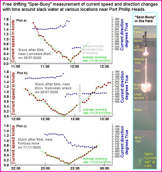
The graph section shows three graphs from runs on different days. These show both the speed of the current (red plot) and its direction (blue plot) over time as the current reversed from ebbing to flooding. This data was derived from the GPS tracker's position record using a 2 minute sampling interval. Slack water time is identified as the bottom of the "V" in the red speed curve, along with the sudden change in the blue curve of the current's direction of flow.
The green lines on the speed plots are used to calculate the rate of change in speed as the current decelerates into slack water and then accelerates away after slack. Within each graph, these gradients are averaged to give the green reversing rate numbers shown in the bottom right hand corner of each plot. I have used the rather unusual units of "knots per 10 minutes" for the rate of speed change numbers simply because this is the most pragmatic and "boating friendly" unit to use near Port Phillip Heads.
The slightly uneven "speed wobbles" seen around the green line are mainly due to slight speed changes of the "water patch" being monitored as it passes over small reef outcrops on the seafloor. This effect is eliminated if suitable speed monitoring equipment could be deployed from a fixed pile of some sort.
The near uniform slope of the "line of best fit" is an interesting outcome of the combination of two forces, one of which shrinks over time as the other grows. Before slack water the frictional drag shrinks as the water slows, but the reverse slope force grows as the reverse level difference increases towards slack water. The two add together to produce a roughly constant slowing force and so a roughly constant slowing rate.
After slack, the frictional drag force grows as the water speeds up, and so does the increasing slope force. However the drag force changed its direction when the flow reversed. So now its growing strength is in the opposite direction to the also growing slope force. The addition of these two growing but oppositely directed forces also yields an approximately constant accelerating force. So the growth in water speed after slack is also roughly constant for that particular slack water event.
The Plot a) location is right at the Heads. The measured reversing rate of +0.36 kn/10min, is 97% of the theoretical Heads reversing rate (+0.37) obtained from the volume modelling work. The Plot b) location is around 4 km inside the Heads. Its measured reversing rate of +0.30 kn/10min is 83% of the theoretical Heads reversing rate for that slack (+0.36). The Plot c) location is about 8 km inside the Heads. Its measured reversing rate of +0.22 kn/10min is 54% of the theoretical Heads reversing rate for that day (+0.41).
These figures show that moving inside the Heads, the expanding underwater cross-section of the Bay not only reduces the maximum tidal stream speeds at the more distant locations, but also their reversing rates. This also shows up in graphs a) to c) as a "widening of the Vs" as the distance inside the Heads increases.
The positive direction for entrance currents in taken as inwards meaning flooding currents are treated as having +ve velocities and ebbing currents as having -ve velocities. Thus a "slack after flood" refers to a reversal where the old flood current and the new reversed ebb current "both become more -ve over time", so the speed change rate takes a negative sign. In a "slack after ebb" reversal, the old ebb current and the new flood current "both become more +ve over time" and so are given a +ve speed change rate.
Under this same direction convention, a +ve surface slope is one that increases in height moving inwards from the Heads. The down-slope force so created is then directed outward though the Heads, so yielding negative speed change rates. A -ve surface slope is one that decreases in height while moving inward from the Heads. In this case the down-slope force so created is directed inward through the Heads, so yielding positive speed change rates.
To convert these reversal rates into sea surface slopes, we need to first convert the speed figures in knots into units of m/s. Then we divide by 600 (600sec=10mins) to give the speed change rate in m/s/s. Then by dividing by "g" = 9.8 m/s/s, we get the speed change rate as a decimal fraction of the acceleration rate of "1g" that all free falling objects experience in the Earth's gravitational field.
Multiplying these small fractional speed change rates in units of "g" by -100,000 then converts these into a "sensibly sized" slope unit of centimetres of height change per kilometre of distance (cm/km).
At location a) [ The Heads ], +0.36 kn/10min = [(+0.36x1853/3600)/600]/9.8 = +0.000032g. Or for the slope in cm/km = +0.000032 x -100,000 = -3.2 cm/km
At location b) [ 4km inside ], +0.30 kn/10min = [(+0.30x1853/3600)/600]/9.8 = +0.000026g. Or for the slope in cm/km = +0.000026 x -100,000 = -2.6 cm/km
At location c) [ 8km inside ], +0.22 kn/10min = [(+0.22x1853/3600)/600]/9.8 = +0.000019g. Or for the slope in cm/km = +0.000019 x -100,000 = -1.9 cm/km
The fixed number parts of the above calculations can be pre-calculated into a single numerical conversion factor to go from acceleration rates in kn/10min to surface slopes in cm/km which is:-
Reversal rate in units of kn/10min x -8.75 = Surface Slope in units of cm/km
A scan of the Heads reversal rates given by the volume modelling method for all 2024 slack water predictions shows the highest reversal rate is -0.64 kn/10min (or +5.6 cm/km). The lowest reversal rate found is +0.14 kn/10min (or -1.2 cm/km).
This wide range of possible reversing rates for a Port Phillip Heads tidal stream suggests that publishing them along side the usual reversal times would give recreational boaters a better idea of which reversals might be "quick" needing much care over timing, and which will be "slow" and much more leisurely. The rates need not be in the rather nerdy "knots/10minutes" units, which might confuse many, but perhaps presented just as a single digit (1 --> 6) as a "speed of reversal" indicator. A footnote might be used to convey a fuller meaning for those wanting more detail.
Readings from the tide gauge network allow the average sea surface slope over the important "Choke Zone" region to be determined at any time. The "Spar Buoy" type of equipment allows the particular slack water sea surface slope at any point to be determined independent of any height measurements. Are the two results compatible?
The results and analysis that follow are not quite as robust as I would like, but it is difficult for a "citizen scientist" to gather the large number of separate measurements required to make the case perfectly watertight. The red plot in the image below portrays how the surface slope at slack water after an ebb tide might vary from 5 km outside the Heads to +15 km inside the Heads.
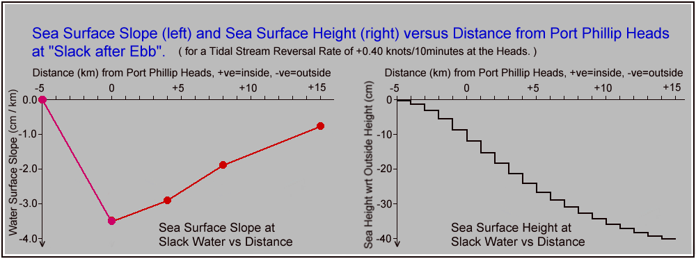
The middle 3 red plot points were obtained using the previous Spar Buoy results that showed the surface slope behaviour at the Heads, the +4 km inside point, and then the +8 km inside point. The -5 km (outside) plot point is based on there being no surface slope at this distance outside the Heads at slack water time. The +15 km plot point is based on the knowledge that at the north east edge of The Great Sands the underwater cross-section of the Bay is around four times larger than that at the Heads. This means both the current speed and the speed change rates are around one quarter of those at the Heads.
Note the surface slopes are negative values, meaning the sea height decreases with distance as we move from Bass Strait into the Main body of the Bay. Note this decrease in height is really an uphill slope from the perspective of the outward flowing ebb stream that has just been halted to give this slack water.
The right side "step plot" (in black) is obtained by progressively adding together the average red plot slope value for each kilometre of distance starting from the -5 km "outside" point and moving towards the +15 km "inside" point. So the resulting "downward staircase" plot represents the progressive level change from "outside" to "inside" at slack water after a moderately strong ebbing tide has been halted. Note that the "step size" is largest around the Heads where the slope hits its steepest value of -3.4 cm/km. We could mentally smooth out this plot to more accurately represent how the sea level at "slack after ebb" drops as we move inside the Heads and across the "choke zone".
Note that the total height drop of around 38 cm from the "outside" to the "inside" zone is entirely consistent with the height data obtained from the tide gauge network (Image #17: slack water events #1 & #3). When properly analysed, all the academic papers published about the "outside" to "inside" level differences that I have examined show a similar result, despite this often being overlooked by the paper's author because in many cases the focus of the paper was not on the slack water period.
There is in fact NO scientific evidence whatsoever to support Ports Victoria's claim (and from many other quarters) that there is no level difference at slack water time. Only when the true behaviour, that a relatively large reverse level difference does exist at slack water becomes more widely accepted, will the majority of recreational boaters understand why the current strength is changing quite rapidly around slack water time, and not slowly as they might have assumed from the untrue official claims. This better understanding of the real current vs time profile should help keep folk safer while boating at or near the Heads around slack water time.
Looking at the Heads current speed curve in Plot a) in the previous pink bordered image, it is hard not to think: "Gee wouldn't it be great to have a real time Heads current plot available online 24/7". It would be particularly comforting for inbound yachtsmen in bad weather and with the uncertainty of how this might affect the slack water time. At Lakes Entrance, where the large Gippsland Lakes system opens into Bass Strait, such a system has been in place for a number of years. I understand its data is very much appreciated by commercial and amateur fishers alike, as well as skippers of visiting yachts and power cruisers.
The instrument making all this possible is an Acoustic Doppler Current Profiler (or ADCP). It uses several divergent ultrasonic beams that shoot sideways across the entrance channel between the breakwaters. With a lot of fancy analysis, it senses small frequency shifts in the backscatter echoes received from small air bubbles and other sound reflectors carried along in the current stream. Using three or four sensor beams it can determine the current's speed and direction at selected distances right across the channel. Could we dream of a similar system for Port Phillip Heads?
Big swells, high waves, and the strong wind conditions that regularly occur at Port Phillip Heads means that is a very rugged place to attempt to insert a fixed current measuring device. Not only are there huge surges back and forth that can rip any bottom mounted device from its moorings, but large pieces of the relatively soft rock on Rip Bank can be broken off and later rolled around in the strong currents rather like a steamroller. There have been many expensive ADCPs damaged, destroyed, or simply lost during a sustained effort to "instrument" Port Phillip Heads.
So at present there are no real current measurements done on a continuing basis at Port Phillip Heads. Instead the behaviour of the entrance current is inferred from various models that use the tide curves (predicted or observed) available for several "inside" and "outside" locations. The image below shows the time behaviour of the predicted tides at several locations, plus the entrance current plot (gold) derived from a water volume model. The times of Maximum Current, Equal Levels, and Slack Water are marked by vertical lines.
The simplest of all slack water prediction algorithms is "The Fishermen's". It ignores all tide curves except for the Williamstown curve which is known to closely represent large areas in the "main body" of the Bay. That algorithm simply says: "High (or Low) tide at Williamstown marks when the Bay is Full (or Empty), and so marks slack water time at the Heads." While that timing is sometimes near enough, it ignores the tides south of the Great Sands, all of which are undergoing fast changes at the time of Williamstown High/Low. The effect of these changes is to pull the real "Full" / "Empty" times somewhat before the Williamstown High / Low times.
The tidal stream speeds given out to ships and recreational yachts by the Vessel Traffic Service (VTS) officers come from a much more complicated algorithm developed many years ago. A key aspect of that algorithm is the use of the level difference between the Lorne and Queenscliff tide gauges. I believe there is also some input from one of the more "inside" gauge locations but I am unaware of the those details.
Note that at the "Max Current" times, the Lorne - Queenscliff level difference (red minus dark blue) represents well over 50% of the total "outside" - "inside" level difference (red minus light blue). However between the "Equal Levels" and the "Slack Water" times, that percentage drops below 50% of the total level difference. The image shows that the red minus light blue level difference might have been a better choice for driving the algorithm, particularly for the weaker tide cycles where the (red minus dark blue) difference can shrink to as little as 15% of the (red minus light blue) difference.
It appears other factors might be at play. In particular both the Lorne and Queenscliff locations are well protected from NW to SW, the most common directions for gales. In addition both locations are accessible from the land so any maintenance or calibration checks are much easier to perform than if a mid-water location was chosen.
There are actually two "flavours" of current speed numbers available from the VTS officers. The first is usually called the "predicted current", with numbers coming from the algorithm when it is feed with the predicted tide curves. These are worked out a year or more in advance, and of course those results can't take account of the weather conditions on the day. The second "flavour" is often called the "measured current" by the VTS folk, even though the word "measured" here really only refers to "measured tide heights". These are then fed into the same algorithm as before. This is an attempt to account for the effects of the weather on currents and slack water times. There are mixed reports as to how effective this technique is.
Short term real current measurements in "The Rip" have been successfully done, but those numbers remain stored within the device until it is later recovered and that data extracted for analysis. Near real-time measurements would also need some above water infrastructure including a radio component that can immediately send the data to a shore based receiving point from where it can be made available to those who need to see it. This infrastructure might create a greater navigational risk than the benefit such a system could provide.
However, comparing the earlier red current speed curves from Plot a) and Plot b), shows that monitoring the current in real time at a location 4 to 5 km inside the Heads would still be very useful. At that distance inside the Heads, swell and wave conditions are not nearly so rough and yet the current strength is still a large fraction of that at the Heads. Importantly the delay of slack water reaching such a location is just one or two minutes. My 2022 submission to the Harbour Master, while mainly grizzling about untrue tidal stream claims, also included the suggestion that real-time current monitoring would seem quite doable at "Entrance Beacon", a prominent fixed steel pile about 5km inside the Heads and at the start of the South Channel.
Not sure if this was taken any note of, or if Ports Victoria later independently also thought this might be a good idea. In any case equipment to provide "live" current strength and direction readings was installed at Entrance Beacon in March 2024. I was told at the time that it might take some months for the remote monitoring system to be ready, but it was likely that these data would be available on request via the VTS officers.
Unfortunately, several requests for those numbers during October and November 2024 drew a blank, as the VTS officers could not locate the relevant graph plots on their screens. Sadly it turned out that while the system had been delivering data for some months after its installation, it had gone off-line in early October due to some unspecified technical issue. There was no date given for the system to return to operation, but it was said this would involve a diver recovery of the bottom mounted instrument, rectification of the problem, and then returning the ADCP to its mooring on the bottom of the sea floor.
(Update: In a further blow to this project, an NtoM on 16/4/2025 announced "Entrance Beacon Destroyed". It didn't say if it was run down by a vessel or knocked over by the current. I suspect it was the latter because I also noted a replacement program for all South Channel beacons was announced in November 2024, so they must of known they were at the end of their service life. The affect on the ADCP real-time current monitoring project at Entrance Beacon is not clear yet but presumably several more months of delay depending on what damage was done to this equipment and its infrastructure.)
An ADCP is a sophisticated and expensive piece of equipment. Long term deployments at remote locations create issues of bio-fouling of the sensors and the continuous supply of sufficient electrical power. Maintenance costs and difficulty are expected to be an ongoing issue.
There is also an issue related to the ADCP's mode of operation. It senses tiny (doppler) frequency shifts in the return echos reflected from tiny air bubbles carried along in the tidal stream. It is rather like the pitch of a speeding ambulance siren appearing to shift down as it passes by. In theory, by measuring that change in frequency, you could calculate the speed the ambulance was travelling at.
The problem for an ADCP is that as well as tiny air bubbles carried along in the tidal stream, there are also more active sound reflectors such as small shrimps and "sea fleas" that also return echos. These sources don't just quietly drift along in the tidal stream, but can actively "flit about" in all sorts of short random movements. Their erratic doppler shift signals need to be removed so that the genuine echos from reflectors only drifting along with the tide stream are not corrupted.
This is usually achieved by averaging out the frequency shifts over say a 10 minute period, on the assumption that the "flitting too and fro" of live biological reflectors would average out as close to zero over that "integration time". Normally this scheme works well, but in this application the rather rapid change in current speed around slack water (approx. 0.5 kn/10min) means ADCP measurements may not have the time resolution to accurately detect the real time of slack water.
Other types of current measuring technologies, such as a "sing-around" ultrasonic velocimeter, or even basic paddle-wheel type devices for current measurement do not have these timing issues. They are much cheaper and could also be deployed on a detachable pole protruding down into the water column. This would give easier surface based access for maintenance and biofouling removal. These cheap devices could also allow a quick "swap over" maintenance regime, without the need for expensive diving operations.
All that being said, an ADCP is considered "the gold standard" equipment for measuring water speeds. Not only is it more accurate, but a bottom mounted ADCP can provide a current speed profile up through almost the entire water column, in contrast to the simpler "single depth" current measuring devices.
From conversations with upper level VTS people, I understand their intent is to rely on a number of medium term ADCP deployments at the Heads and other places in order to better understand the relationship of the currents along the main shipping leads to those at the new monitoring station at Entrance Beacon. Once that relationship is determined, they can then use the data from Entrance Beacon to project what the mid-channel currents are at the Heads. That is an ambitious project and will take quite some time.
I think the end goal is to move away from the "algorithm estimates" of the entrance currents and move to a system based around actual near-real-time current measurements. When this is achieved it should remove all the weather uncertainties from the present VTS entrance current advice to ship masters and recreational skippers. They could also advise on the expected current reversal rate around the slack water window. Both these things would be a boost to the safe navigation of all types of craft at and near Port Phillip Heads. It may also lead to improvements in any prediction algorithms for the entrance current, which will still have to be available as a backup system. We all just have to show some patience as this ambitious project unfolds!
If you arrived here by following a link from the Index Page, just close this page to return to the Index to see the other links to related posts.
If you arrived here via an external link, you can visit the site's Index Page with this link: Jake's Index Page
--------------------------------- The End ----------------------------------